Data assimilation for Glacier Modeling

This post was written by Emily Corcoran, Hannah Park-Kaufmann, and Logan Knudsen. The project was advised by Dr. Talea Mayo. Our team has also created a midterm presentation, blitz video, poster, paper, and has published their code.

Glaciers

Research has shown that climate change will likely impact storm surge inundation and make modeling this process more difficult. Sea-level rise caused by climate change plays a part in this impact. To better model sea-level rise, glaciers can be modeled. Marine-Terminating Glaciers have a natural flow towards the ocean, which contributes to sea level rise. By the year 2300, the Antarctic ice sheet is projected to cause up to 3 meters of sea level rise globally. Due to the severe impacts of glacial melting, modeling changes in ice sheets is an important task. There are challenges to modeling sea level rise, as ice sheet instability leads to significant sea-level rise uncertainty.

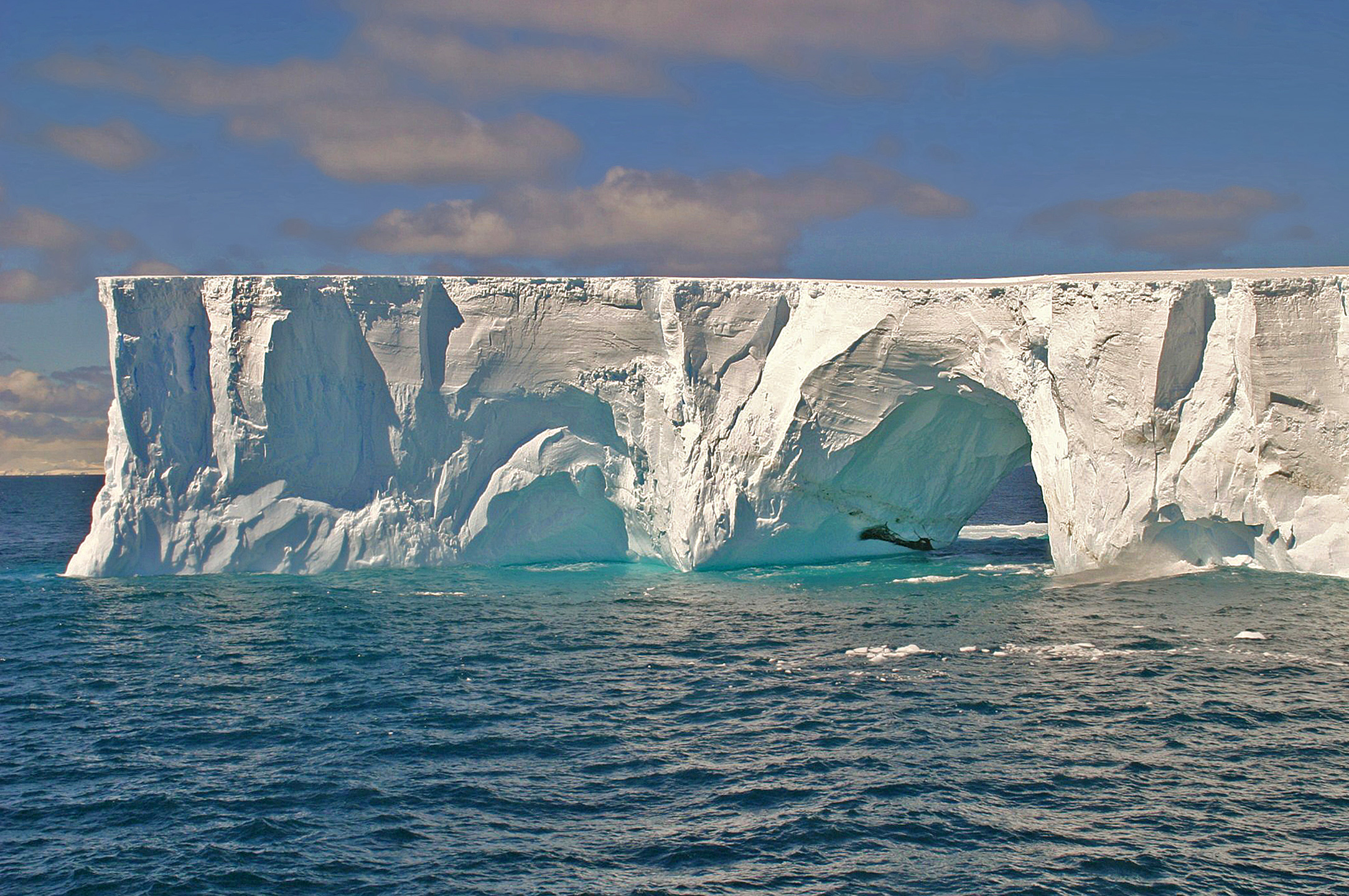
Image by W. Bulach, used under Creative Commons Attribution-Share Alike 4.0 International License

Modeling Glaciers

Our group is collaborating with Dr. Robel, a glaciologist, climate scientist, and applied mathematician from Georgia Tech, and working with the glacier model described in his 2018 paper. This ice sheet model aims to describe the changes in ice mass of marine-terminating glaciers, which may be impacted over time by climate change.

Image used with permission from Dr. Alexander Robel

A glacier can be represented with a simplified box model that has a length $L$, precipitation $P$, and height and flux at the grounding line $h_g$ and $Q_g$. This model is the best approximation for one variable and describes the dominant mode of the glacial system.

The two-stage model that our group is using incorporates a nested box into the system. This new box has a thickness, $H$, and an interior flux, $Q$. The change in length and height of the glacier can be described with these differential equations: $$\ \dfrac{dH}{dt}=P-\dfrac{Q_g}{L}-\dfrac{H}{h_gL}(Q-Q_g)$$ $$\ \dfrac{dL}{dt}=\dfrac{1}{h_g}(Q-Q_g)$$

Sensitivity Analysis

Sensitivity analyses study how various sources of uncertainty in a mathematical model contribute to the model’s overall uncertainty. This allows us to understand the model better.

Why do we do this? Why do we care about the uncertainty of a model? And where do the uncertainties even come from? In this ice sheet model, just like in any model, there are always going to be simplifications, and these lead to uncertainties. We need to have a good idea of which uncertainties matter the most, so that we better know the limits of where our model does a good job of simulating the real world.

The basic idea is this: We check sensitivity by using different distributions for the input parameters. If the outputs vary significantly, then the output is sensitive to the specification of the input distributions. Hence these should be defined with particular care. We can also look at the sensitivity of the model parameters to inform which parameter we’re going to work with in the data assimilation. We want to be working with the most sensitive parameter, because it has the most promise for things we vary later on to matter, in questions like: “if your data is from billions of years ago does that matter? Is it important to have your data from the last 60 years?” or “how much will noise impact the predictions?”

The uncertain model parameters we considered are: initial conditions, sill parameters, and SMB values. For consistency’s sake, we vary each parameter by +-10 percent of the nominal values originally given in our model code. Below you can see three graphs, one for each group of parameters varied, for each “time vs H(t)” (Height of the glacier at time) and “time vs L(t)” (Length of the glacier at time).

Looking at the distributions, we see that varying initial conditions (Leftmost) seems to produce the greatest spread, but the slopes of the lines there are all very similar. Varying the sill parameters (Middle) produces a lesser spread than varying initial conditions, however there is a greater variation in the slope of the lines. Finally, when varying the smb data (Rightmost) the result actually doesn’t change that much and is quite stable. Thus, according to our analysis, the model is the least sensitive to SMB parameters, and between initial and sill parameters judgement varies depending on what you care about more - spread or slope.

Data Assimilation

Data assimilation is a method to move models closer to reality using real world observations by readjusting the model state at specified times.

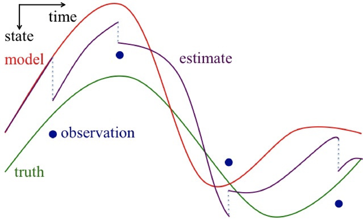
Image used with permission from Dr. Talea Mayo.

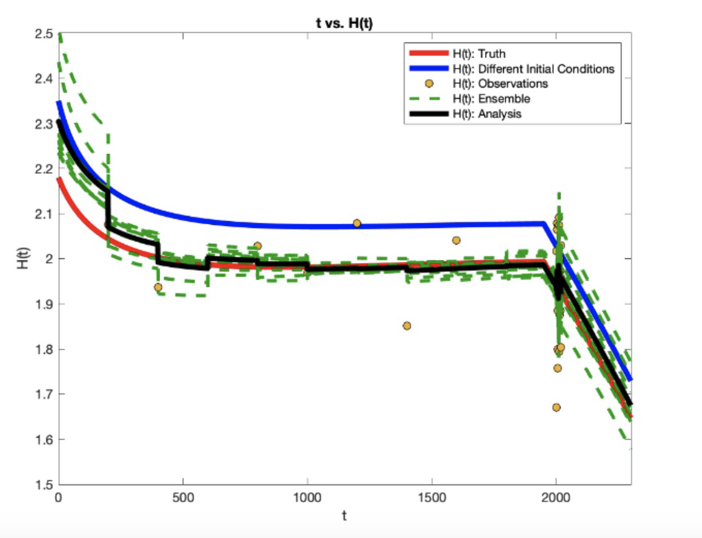
In this example we have used the ensemble Kalman filter method (ENKF) in order to perform our data assimilation. In basic terms, we initialize an ensemble( or a series of model runs with perturbed initial conditions) and performed data assimilation on each of the ensemble members, then to get our final analysis we took the mean of the ensemble.

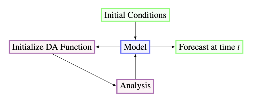
The program used to model the glacier behavior and assimilate the data begins with choosing a set of initial conditions. Once the initial conditions are input to the model, which after taking a step using a Runge-Kutta 4th Order Method, is plugged into a Data Assimilation Method. Our main method is ENKF as previously mdentioned. Finally, the analyzed data from the assimilation is output and plugged back into the model. It should be noted that at sometimes the forecast output for the model is the same as the analyzed data.

Square Difference

The error measure we use in the best ensemble size and observation scheme is the square difference, $d^2$, which we define $$\ d_t^2 = \left(x_t - x^a_t\right)^2 $$ where $x_t$ is the true state from the truth simulation at time $t$ and $x^a_t$ is the analysis state at time $t$.

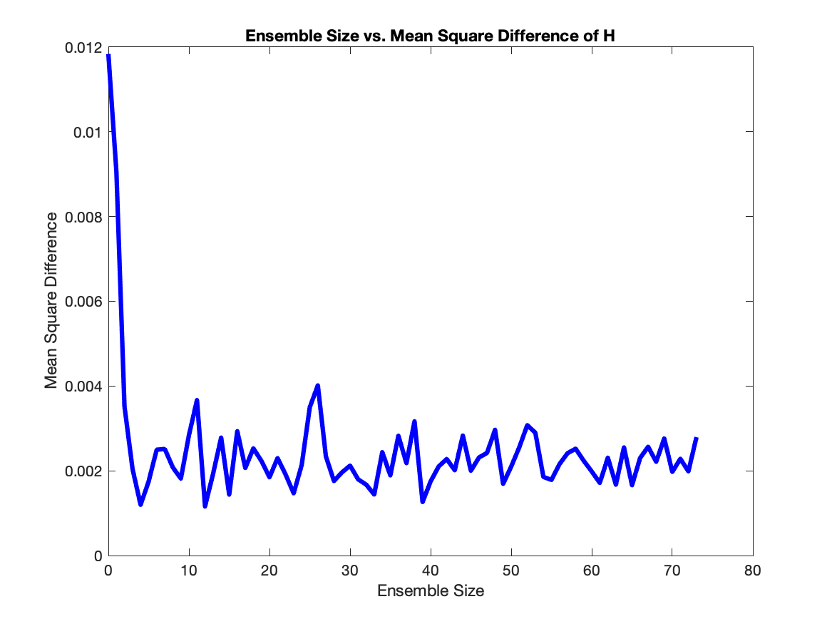
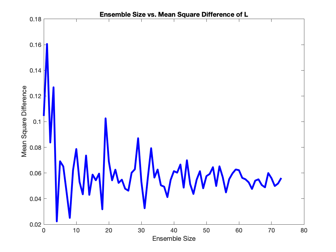
Ensemble Size

In the interest of lowering computational costs, we use the square difference in order to minimize ensemble size while also minimizing error. To do this, we choose an ensemble size, calculate the square difference at each $t$, and then calculated the mean of all these square differences. We ran this calculation for ensembles sizes from 2 up to 75, and found that ensembles of size 7-10 were ideal as they were at the point where the average square difference hovers around the same value.

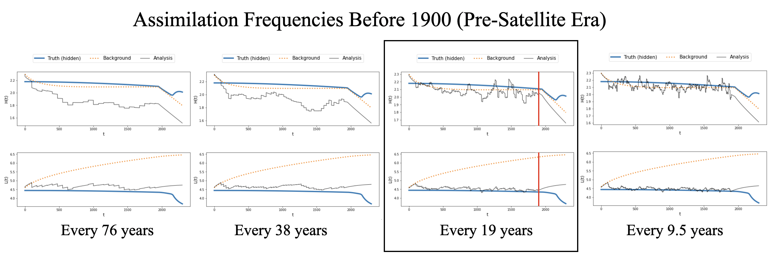
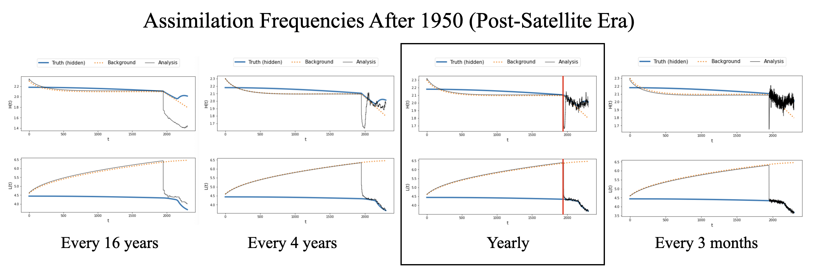
Observation Scheme

We ran the model for various observation schemes to find the best observation scheme, i.e. the times frames and frequencies which can produce a sufficiently small average square difference over the course of the model run. We applied this process to our model and found that for before 1900 the best observation frequency, while still using small number of observations, would be every 19 years for a total of 100 observations. Similarly, for the time frame of 1950-2300 we found that yearly observations for a total of 350 observations is the best frequency.

Model Runs

Using the facts we established in the previous two sections, we ran the model using EnKF for the time frame of 0-2022 in order to project $H$ and $L$ into the future up to the year 2300. The following plots show the results of this experiment, which we will use to help calculate $Q$ and $Q_g$ over time, and in turn use it to calculate sea level rise.

Sea Level Rise

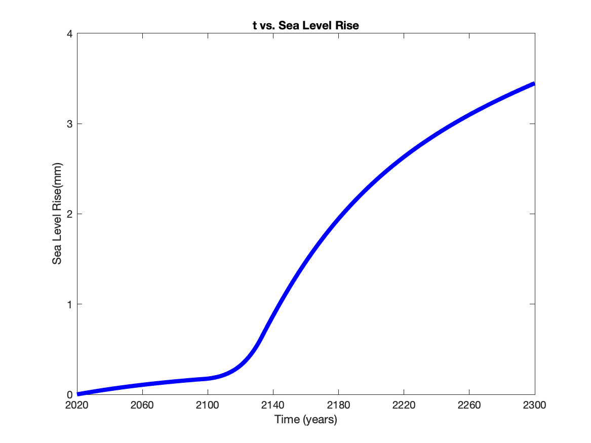
Using the formulas for $Q$ and $Q_g$ we can calculate the volume lost across the grounding line $$\ V_{gz} = W(Q-Q_g)t $$ We then used the to calculate the volume out at all times and add it up to get accumulated volume loss. We then assume that the width of the glacier is 50 km(at least in the case we show here). To convert this to sea level rise, note that 394.67 km$^3$ of ice is equivalent $1$ mm of sea level and get the following projection of sea level rise.

Next Steps

Using data assimilation can help to inform the glacier modelers and glaciologists who collect data about how to collect data in an efficient way. This can help researchers to more efficiently utilize funding and avoid unnecessarily expensive data collection that does not significantly improve glacier models. Data assimilation should be explored within more complicated glacier models, as the model used here is quite simplified. If more research is performed on this technique, it could greatly improve the practice of glacier modeling. Data assimilation can also be used for many geophysical modeling tasks, such as weather forcasting and hurricane storm surge modeling. Going forward, we plan to integrate the output of the glacier model into the ADCIRC hurricane storm surge model to predict the impact of glacier model on storm surge inundation.

References

The long future of Antarctic melting
Marine ice sheet instability amplifies and skews uncertainty in projections of future sea-level rise
Projected climate change impacts on hurricane storm surge inundation in the coastal United States
Response of marine-terminating glaciers to forcing: time scales, sensitivities, instabilities, and stochastic dynamics

About the Team

Emily Corcoran

Emily Corcoran is a junior at New Jersey Institute of Technology, majoring in Mathematical Sciences with a concentration in Applied Statistics and Data Analysis. Before this REU, she has worked as a research assistant in her school’s Visual Perception Lab. She is a student in the Albert Dorman Honors College and is an active member of NJIT’s school yearbook and Knit ’n Crochet club. When she is not in class, she can be found reading, listening to music, or attending a local play.

Logan Knudsen

Logan Knudsen is a senior at Texas A&M University majoring in Mathematics with minors in Oceanography and Meteorology. Before this REU, he has worked doing research on Data Analysis using Benford’s Law and as a Teaching Assistant. Logan is currently the President of Texas A&M’s Math Club and a member of student radio, KANM. When not in class, he can be found reading, playing the guitar or playing video games with his friends.

Hannah Park-Kaufmann

Hannah Park-Kaufmann is a junior at Bard College and Conservatory, majoring in Mathematics and Piano Performance. Before this REU, she conducted research on Numerical Semigroups and Polyhedra, and on Identifying Universal Traits in Healthy Pianistic Posture using Depth Data. She tutors math in the Bard Prison Initiative (BPI). When not doing math, she can be found playing piano, reading scores, reading literature and/or eating.