Optimization for Economics, a Visual Approach

Mike Carr

Contents

0 Calculus Reference 3

0.1 Graphs of Functions . . . . . . . . . . . . . . . . . . . . . . . . . . . . . . . . . . . . . 4

0.2 Limits and Derivatives . . . . . . . . . . . . . . . . . . . . . . . . . . . . . . . . . . . . 10

0.3 Multivariable Functions . . . . . . . . . . . . . . . . . . . . . . . . . . . . . . . . . . . 19

1 Unconstrained Optimization 31

1.1 Single-Variable Optimization . . . . . . . . . . . . . . . . . . . . . . . . . . . . . . . . 32

1.2 Concavity . . . . . . . . . . . . . . . . . . . . . . . . . . . . . . . . . . . . . . . . . . 48

1.3 Multivariable Optimization . . . . . . . . . . . . . . . . . . . . . . . . . . . . . . . . . 68

2 Constrained Optimization 89

2.1 Equality Constraints . . . . . . . . . . . . . . . . . . . . . . . . . . . . . . . . . . . . . 90

2.2 Inequality Constraints . . . . . . . . . . . . . . . . . . . . . . . . . . . . . . . . . . . . 106

2.3 The Kuhn-Tucker Conditions . . . . . . . . . . . . . . . . . . . . . . . . . . . . . . . . 116

3 Comparative Statics 135

3.1 The Implicit Function Theorem . . . . . . . . . . . . . . . . . . . . . . . . . . . . . . . 136

3.2 The Envelope Theorem . . . . . . . . . . . . . . . . . . . . . . . . . . . . . . . . . . . 154

4 Suﬃcient Conditions 163

4.1 The Extreme Value Theorem . . . . . . . . . . . . . . . . . . . . . . . . . . . . . . . . 164

4.2 The Bordered Hessian . . . . . . . . . . . . . . . . . . . . . . . . . . . . . . . . . . . . 173

4.3 Separation . . . . . . . . . . . . . . . . . . . . . . . . . . . . . . . . . . . . . . . . . . 178

4.4 Concave Programming . . . . . . . . . . . . . . . . . . . . . . . . . . . . . . . . . . . 186

4.5 Quasiconcavity . . . . . . . . . . . . . . . . . . . . . . . . . . . . . . . . . . . . . . . . 201

Note to the Reader

For the last several years I have taught a course in optimization at Emory University for seniors

majoring in mathematics and economics. While mathematics and economics is the standard preparation

for a doctoral program in economics, the vast majority of students in this course are bound for careers

in ﬁnance. One of the challenges in designing this course has been balancing the interests and needs

of students on both tracks. These notes have evolved from my own teaching materials. Their goal is

to present methods for optimization and the reasoning behind them. This reasoning makes students

resilient to the myriad modiﬁcations that these tools endure at the hands of economists.

As an outsider to economics education, I was impressed to see the extent to which economics has

embraced visual methods of instruction. More than any other ﬁeld whose foundation lies in mathematics,

the standard economics curriculum provides students not only with descriptions and formulas, but with

diagrams to depict core principles. Microeconomics students are inundated with supply curves, budget

lines, indiﬀerence curves, and graphs in marginal space. This is certainly a lifeline for visual learners,

but I suspect it produces deeper understanding for all.

As a geometer, my ﬁrst inclination is to lean heavily upon visual reasoning when presenting the

methods of optimization. In our eﬀorts to ﬁnd a textbook for our admittedly niche curriculum, we have

not found a economics-focused text that takes this approach. I have made these notes available in the

hope that this visual viewpoint can become an eﬀective supplement to existing techniques. Like with

the graphical arguments in undergraduate microeconomics, I think it can bring a complete and rigorous

understanding of optimization methods to a broader set of learners.

The audience for this text is anyone who wants to understand the mathematical methods for ﬁnding

maximizers in economic theory. The best-prepared reader will have mastered the techniques of diﬀer-

entiation, including partial derivatives. They will also be familiar with the foundations of mathematical

logic: set notation, functions, and methods of proof like contradiction and the contrapostive. Finally,

they will need a basic proﬁciency in vector and matrix operations: sums, products and determinants. A

competent high-school treatment may suﬃce for this requirement.

Anyone who sets out to teach or learn the methods of optimization from this text should be aware

of its limitations. It does not contain the economic applications that my economist colleagues present

each semester. These must be provided in order to create genuine enthusiasm for the material. This is

a deﬁciency that I would like to rectify eventually, if there is some consensus about which examples to

include.

We have used one widely-available source of economic examples: Optimization for Economic Theory

by Avinash Dixit. This excellent book has a rigorous, traditional treatment of most of the material here

and good explanations of some advanced applications. Dixit’s book has proved too diﬃcult for all but the

strongest undergraduates to read independently, but the examples are compelling and comprehensible

with some extra exposition.

Finally I would like to acknowledge my economist colleagues Blake Allison and Teddy Kim who were

essential partners in developing this course. Three students, Alexia Witthaus, Jacob Sugarmann and

Aarya Aamer, carefully read my early drafts and asked many questions. Their feedback allowed me to

identify the most opaque exposition (and clarify it, I hope). There is still a long road of revision and

improvement ahead for this document. I would appreciate any feedback you have.

Mike Carr

May 2023

Chapter 0

Calculus Reference

0.1

Graphs of Functions

Goals:

1 Graph algebraic functions.

2 Graph transformations of functions.

0.1.1

Graphs of Basic Functions

Deﬁnition 0.1

The graph of a function f(x) is the set of points (x, y) whose coordinates satisfy the equation y = f(x).

In this section we review several basic functions and their graphs. These will be important as examples

and counterexamples for our methods of optimization. In addition, knowing the shape of a graph is an

eﬃcient way to memorize the behavior of functions that appear frequently in economic models.

Deﬁnition 0.2

Linear functions can be written in slope-intercept form:

f(x) = mx + b.

The graph of a linear function is a line.

m is the slope, which is the change in y over the change in x between any two points on the line.

(0, b) is the y intercept.

If we have the slope and a known point (a, b) on a line. We can write its equation in point-slope

form.

y − b = m(x − a)

Deﬁnition 0.3

A monomial is a function of the form:

f(x) = x

where n is an integer greater than 0.

For n ≥ 2 the graph y = x

curves upward over the positive values of x.

Greater values of n have lower values of f(x) when 0 < x < 1 but higher values when x > 1.

For even values of n the graph is symmetric across the y-axis, curving up when x is negative.

For odd values of n the graph curves down when x is negative. It is anti-symmetric across the

x = 0.

Figure 1: Graphs of even-powered

monomials

Figure 2: Graphs of odd-powered

monomials

Monomials of Negative Power

Monomials of negative power have the form f (x) = x

−n

. They are also commonly written

f(x) =

The graph y =

has a vertical asymptote at x = 0.

The graph approaches the x-axis, y = 0 as x gets large.

For even values of n, the graph is above the x-axis.

For odd values of n, the graph is above the x-axis for positive x and below it for negative x.

A greater choice of n makes the function approach the x-axis more quickly.

0.1.1

Graphs of Basic Functions

Figure 3: Graphs of y = x

−2

, y = x

−4

and y = x

−6

Figure 4: Graphs of y = x

−1

, y = x

−3

and y = x

−5

Deﬁnition 0.4

A root function is a function of the form:

f(x) =

√

where n is an integer greater than 0.

The domain of

√

x is [0, ∞) if n is even and all real numbers if n is odd.

The x and y intercept of y =

√

x is at (0, 0).

Root functions are increasing. At x = 0, they travel straight up.

√

Figure 5: Graphs of root functions

Deﬁnition 0.5

An exponential function has the form:

f(x) = a

where a is a number greater than 0.

a is called the base of the exponential function.

The graph y = a

passes through (0, 1).

If a > 1 then f(x) increases quickly as x takes on positive values. Greater values of a give a

steeper increase. f(x) approaches 0 as x goes to −∞. Greater values of a give a faster approach.

The graph does not touch or cross the x-axis.

If a < 1, then the above is reversed.

e is a commonly used base. e is approximately 2.718.

Figure 6: Graphs of y = 2

, y = e

and y = 3

Deﬁnition 0.6

A logarithmic function has the form:

f(x) = log

where the base a is a number greater than 1. log

x is the number b such that a

= x. The natural

logarithm is the logarithm with base e. It is denoted f (x) = ln x.

can never be 0 or less. The domain of f(x) = log

x is (0, ∞).

As x approaches 0, log

x goes to −∞.

y = log

x has an x intercept at (1, 0).

0.1.1

Graphs of Basic Functions

y = log

x grows more and more slowly as x increases. This eﬀect is more pronounced for larger

values of a.

Figure 7: Graphs of y = log

x, y = ln x and y = log

Logarithms and exponents are inverse functions. We solve exponential equations by applying a

logarithm to both sides. We solve logarithm equations by exponentiating both sides.

= c x = log

log

x = c x = a

0.1.2

Graphs of Transformations

Suppose we would like to transform the graph y = f(x). Here are four ways we can.

The graph of y = af(x) is stretched by a factor of a in the y direction.

The graph of y = f(x) + b is shifted by b in the positive y direction.

The graph of y = f(cx) is compressed by a factor of c in the x direction.

The graph of y = f(x + d) is shifted by d in the negative x direction.

We can perform multiple transformations on a single function.

Figure 8: The graph of y = f (x) and its transformation y = af (cx + d) + b

0.2

Limits and Derivatives

Goals:

1 Verify that a function is continuous.

2 Compute derivatives.

3 Use derivatives to understand graphs and vice versa.

0.2.1

The Limit of A Function

Calculus is the study of change. Our most important rate of change cannot be computed directly,

but exists only as a limit of rates.

Deﬁnition 0.7

The limit as x approaches a (or x → a) of a function f(x) is denoted lim

x→a

f(x).

lim

x→a

f(x) = L means that we can make f(x) arbitrarily close to L by restricting x to a small

enough neighborhood surrounding a.

If there is no L such that lim

x→a

f(x) = L, we say that lim

x→a

f(x) does not exist.

Remark

arbitrarily close means any amount of closeness demanded. We need to be able to make f(x)

within

of L, within

1000

of L, within

10000000

of L and so on. When proving that a limit

exists, mathematicians traditionally model this closeness with the variable ϵ. We indicate or verify

arbitrary closeness with the inequality |f (x) − L| < ϵ.

By a neighborhood we mean an open interval that contains a. The set {a} is not a neighborhood.

If it were, then every function would limit to f(a) as x → a. Mathematicians generally restrict to

neighborhoods of the form (a − δ, a + δ), then they need a way to produce a valid, positive δ for

any given positive ϵ.

Figure 9: A neighborhood of a that keeps f(x) within ϵ of L

0.2.2

Continuity

Limits give us a formal approach to deﬁning continuity. Many of our results will rely on the fact that

a function is continuous.

Deﬁnition 0.8

A function f(x) is continuous at a, if

lim

x→a

f(x) = f(a).

f(x) can also be continuous on an interval or other set of points if it is continuous at each a in that

set. If it is continuous on R, we say f(x) is a continuous function.

Proving that a function is continuous requires us to verify its limit at every point a. This is too

much work for a case-by-case basis. Instead mathematics adopts a constructive approach. First we show

that a few basic functions are continuous. Next we prove that sums, diﬀerences, products and other

combinations preserve continuity.

0.2.2

Continuity

Theorem 0.9

The following functions are continuous on their domains

1 Constant functions

2 Linear functions

3 Polynomials

4 Roots

5 Exponential functions

6 Logarithms

7 Trigonometric functions

8 f(x) = |x|

Theorem 0.10

If f(x) and g(x) are continuous on their domains, then the following are also continuous on their

domains

1 f(x) + g(x)

2 f(x) − g(x)

3 f(x)g(x)

f(x)

g(x)

(note that any x where g(x) = 0 is not in the domain)

5 f(x)

g(x)

as long as f(x) > 0

6 f(g(x))

We can use these theorems together to argue that complicated functions are continuous.

Example

The function f(x) =

√

− 17x + 2 −

log

is the diﬀerence of two functions. The ﬁrst is a compo-

sition of a root function and polynomial (both continuous on their domains). The second is a quotient

of an exponential and a logarithm (both continuous on their domains). Thus f(x) is the diﬀerence of

two continuous functions and is continuous on its domain.

Remark

Just about any function we can write using algebraic expressions is continuous on its domain. This does

not mean it is continuous everywhere. f(x) =

is not continuous at x = 0, for example.

0.2.3

The Intermediate Value Theorem

One early intuition for continuity is that the graph of a continuous function can be drawn without

any breaks. There are many ways to formalize this idea. One of the most important is the following

theorem.

Theorem 0.11 [The Intermediate Value Theorem]

If f is a continuous function on [a, b] and K is a number between f(a) and f (b), then there is some

number c between a and b such that f(c) = K.

Intuitively, a continuous graph cannot get from one side of the line y = K to the other without

intersecting y = K. Notice that this theorem does not say exactly where this intersection must occur,

only that it must occur somewhere in the interval (a, b). It also does not rule out the possibility of more

than one such c existing.

Example

Show that f (x) = e

− 3x has a root between 0 and 1.

0.2.3 The Intermediate Value Theorem

Solution

A root is a number c such that f(c) = 0. To prove such a root exists, we check the conditions of the

intermediate value theorem.

f(x) is a sum of continuous functions, so it is continuous on its domain.

f(0) = 1

f(1) = e − 3 < 0

0 is between f(0) and f(1)

We conclude there is some c between 0 and 1 such that f (c) = 0.

−1

1 2

−1

y = e

− 3x

(0, 1)

(1, 3 − e)

Figure 10: A root of y = e

− 3x

0.2.4

The Derivative

The derivative is a method for measuring the rate of change of a function.

Deﬁnition 0.12

Given a function f(x), the derivative of f(x) at a is the number

lim

h→0

f(a + h) − f (a)

The derivative function of f(x) is the function

lim

h→0

f(x + h) − f (x)

Here are two diﬀerent notations for the derivative at a.

(a) (Leibniz)

2 f

′

(a) (Lagrange)

The ratio

f(a + h) − f (a)

can be interpreted two ways

1 The average rate of change of f between a and a + h

2 The slope of a secant line of y = f(x) from (a, f(a)) to (a + h, f(a + h))

Since the derivative is the limit of these, we interpret f

′

(a) as

1 The instantaneous rate of change of f at a

2 The slope of a tangent line to y = f(x) at (a, f(a))

Figure 11: A secant line and a tangent line to y = f (x)

0.2.4

The Derivative

We can take higher order derivatives by taking derivatives of derivatives. The derivative function

of f in this context is called the ﬁrst derivative. Its derivative function is the second derivative. The

second derivative’s derivative function is the third derivative and so on.

Notation

The following notations are used for higher order derivatives

name Lagrange notation Leibniz notation

ﬁrst derivative f

′

(x)

second derivative f

′′

(x)

third derivative f

′′′

(x)

fourth derivative f

(4)

(x)

ﬁfth derivative f

(5)

(x)

The sign of a higher order derivative tells us how the derivative of one order lower is changing. For

example if

< 0, then

is decreasing.

0.2.5

Computing Derivatives

The limit deﬁnition of a derivative is too unwieldy to use every time. Instead calculus students learn

the derivatives of some basic functions. They then use theorems to compute derivatives when those

functions are combined.

Derivatives of Basic Functions

c = 0 (derivative of a constant is 0)

= nx

n−1

for any n = 0 (The Power Rule)

= e

= a

ln a for a > 0

ln x =

log

x =

x ln a

The following rules allow us to diﬀerentiate functions made of simpler functions whose derivative we

already know.

Diﬀerentiation Rules

Sum Rule: (f(x) + g(x))

′

= f

′

(x) + g

′

(x)

Constant Multiple Rule: (cf(x))

′

= cf

′

(x)

Product Rule: (f(x)g(x))

′

= f

′

(x)g(x) + g

′

(x)f(x)

Quotient Rule:



f(x)

g(x)



′

(x)g(x)−g

′

(x)f(x)

(g(x))

unless g(x) = 0

Chain Rule: (f(g(x))

′

= f

′

(g(x))g

′

(x)

0.2.6

Computing a Derivative

Compute

√

75 − 3x

+ 10)

0.2.6

Computing a Derivative

Solution

We begin by computing the ﬁrst derivative. We use the chain rule with 4x

1/2

+ 10 as the outer function

and 75 − 3x

as the inner function.

75 − 3x

+ 10) = 2(75 − 3x

)

−1/2

(−6x)

= −

12x

√

75 − 3x

We compute the second derivative by diﬀerentiating the ﬁrst derivative. We use the quotient rule. We

need the chain rule again when we diﬀerentiate the denominator.

75 − 3x

+ 10) = −

12x

√

75 − 3x

= −

(12x)

√

75 − 3x

−

(

√

75 − 3x

)(12x)

(

√

75 − 3x

)

= −

√

75 − 3x

√

75−3x

(12x)

75 − 3x

= −

√

75 − 3x

36x

√

75−3x

75 − 3x

We can obtain a common denominator to simplify this expression.

75 − 3x

+ 10) = −

12(

√

75−3x

)

√

75−3x

36x

√

75−3x

75 − 3x

= −

12(75 − 3x

) + 36x

(75 − 3x

)

3/2

= −

900

(75 − 3x

)

3/2

0.3

Multivariable Functions

Goals:

1 Compute partial derviatives.

2 Recognize continuous multivariable functions.

3 Apply the chain rule to compositions of multivariable functions.

0.3.1

Multi-Variable Functions

Most interesting phenomena are not described by a single variable. We will need to develop methods

for optimizing multivariable functions. There are many ways to denote multivariable domains and the

functions on them. This is how we will denote them.

Notation

An n-vector is an ordered set of n numbers called components. For instance a = (5, −

√

17, 12.31)

is a 3-vector.

We add a vector arrow, as in a, to indicate that a is a vector.

The components of a vector can be denoted abstractly by subscripts: x = (x

, x

, . . . x

). The

do not have arrows because they are numbers, not vectors.

n-space, the set of all n-dimensional vectors, is denoted R



0 is the zero vector: (0, 0, 0, . . . , 0). The dimension should be clear from context.

The vectors e

, e

, . . . , e

are the standard basis vectors of R

. e

has 1 in the ith component

and 0 in the others. For example e

= (0, 1, 0, . . . , 0).

An n-variable function f (x

, x

, . . . , x

) can be written f(x).

0.3.1

Multi-Variable Functions

Remark

Using a common letter with an index variable

, x

. . .

is a good choice for a large or an unknown number of variables. We will use this notation when developing

the theory of multivariable optimization. In many economics problems, there is a ﬁxed, small number

of variables. In these problems, it is more convenient to use diﬀerent letters for each variable, to avoid

keeping track of subscripts.

x, y, z, . . .

Even better, we should try to choose descriptive variable names like q for quantity or p for price.

We visualize functions with their graphs. The height of the graph over a point in the domain

represents the value of the function at that point. This allows us to detect visually where the function

is large or small, increasing or decreasing.

Deﬁnition 0.13

Given an n-variable function f(x), the graph of f is the set of points (x

, x

, . . . , x

, y) in R

n+1

that

satisfy y = f(x

, x

, . . . , x

Figure 12: The graph y =

36 − 4x

− x

and the height showing f(1, 4).

Remark

In general, a graph of the form y = f (x

, x

) will be hard to visualize. For more than three variables,

this visualization becomes impossible. So why bother? Graphs are a useful visual aid to the reasoning

behind our methods. As we progress, it is useful to have an prototypical two-variable graph in your

head. You can apply our methods to that graph, whether or not you have an algebraic expression to go

with it.

0.3.2

Partial Derivatives

Our optimization tools rely on the ability to measure rates of change. For a function of multiple

variables, there are many rates of change, because there are many ways in which the input variables can

change. The simplest are those where only one variable is changing while the others remain ﬁxed.

Deﬁnition 0.14

The partial derivative of f with respect to x

is a function of x. It measures the rate of change of f

at x as x

increases but the other coordinates remain constant. The formula is

lim

h→0

f(x + he

) − f (x)

Here are two diﬀerent notations for the partial derivative.

∂f

∂x

(x) (Leibniz)

2 f

(x) (Lagrange)

Each has advantages, so we will use both. When it will not cause confusion, we can shorten Lagrange’s

notation from f

(x) to f

(x).

In the two variable case, we can interpret f

(x) as the slope of the tangent line to the graph

y = f(x

, x

) in the x

-direction. Higher-dimensional partial derivatives are also slopes, but are harder

to visualize.

0.3.2

Partial Derivatives

Figure 13: The tangent line to y = f (x

, x

) in the x

-direction

Computing a partial derivative requires us to treat the non-changing variables as constants. Then

we can perform ordinary single-variable diﬀerentiation with the respect to the variable that is changing.

0.3.3

Computing a Partial Derivative

The proﬁt of a ﬁrm with a Cobb-Douglas production function might be modeled by

π(L, K) = pL

− wL − rK.

We can compute the partial derivative π

(L, K), which measures the marginal eﬀect of hiring more

labor.

Solution

Since π

(L, K) is a partial derivative, we can treat K as a constant. That means that neither K

nor

rK is changing. We treat K

as a constant multiple of the monomial function L

. We treat rK as a

constant term with derivative 0.

(L, K) = pαL

α−1

− w

0.3.4

Multivariable Limits and Continuity

Deﬁnition 0.15

A multivariable function f (x) is continuous at a, if

lim

x→a

f(x) = f(a)

In order to verify this limit, we must check that f(x) can be made arbitrarily close to f(a) by

restricting to a suﬃciently small neighborhood of a. This neighborhood allows for travel in inﬁnitely

many directions from a, rather than just forwards and backwards like a one-variable limit. This makes

multivariable limits diﬃcult to compute rigorously and multivariable continuity diﬃcult to verify directly.

Fortunately, we can use the same approach we used for single-variable functions.

Variant of Theorem 0.9

The following multivariable functions are continuous on their domains

1 Constant functions

2 Linear functions

3 Polynomials

4 Roots

5 Exponential functions

6 Logarithms

7 Trigonometric functions

0.3.4 Multivariable Limits and Continuity

Variant of Theorem 0.10

If f(x) and g(x) are continuous on their domains, and c is a constant, then the following are also

continuous on their domains

1 f(x) + g(x)

2 f(x) − g(x)

3 f(x)g(x)

f(x)

g(x)

(note that any x where g(x) = 0 is not in the domain)

5 f(x)

g(x)

as long as f(x) > 0

6 f(g(x)) where f (x) is a one-variable function

Multivariable continuity becomes important when discussing derivatives. Partial derivatives do not

use multivariable limits. They use a limit as a single variable h goes to 0. For this reason, we are not

guaranteed that partial derivatives reliably model the shape of a function.

Example

Consider the function

f(x

, x

) =

(

0 if x

≤ 0

if x

> 0

This function is 0 when x

= 0 or x

= 0. Thus the partial derivatives at (0, 0) are

(0, 0) = 0 f

(0, 0) = 0

If we increase x

while holding x

constant or increase x

while holding x

constant, then the function

stays constant at 0. This does not reﬂect the fact that if we increase both x

and x

at (0, 0), the

function will have a positive slope.

Many theorems rely on a function behaving consistently with its partial derivatives no matter which

direction we travel. The following property will usually serve that purpose.

Deﬁnition 0.16

A function f(x) is continuously diﬀerentiable, if all the partial derivative functions f

(x) are continuous

functions. If instead they are all continuous at a point a, we say f(x) is continuously diﬀerentiable at

a.

0.3.5

The Chain Rule

How do model the change of a multivariable function when more than one input variable is changing?

We write each input variable as a function of a parameter. For instance, if x

and x

are both changing

we can write each as a function of a parameter t. We can combine these to deﬁne a vector function:

x(t) = (x

(t), x

(t)).

f(x(t)) is a composition of functions. If we have deﬁned x

(t) and x

(t) to correctly model the change

we want in x

and x

, then the derivative of f(x(t)) will tell us how f is changing as well. Notice

f(x(t)) is a single variable function. The value of t determines its value completely. The multivariable

chain rule computes its derivative using x(t) and the gradient of f(x).

Deﬁnition 0.17

Given a function f(x), the gradient vector of f at x is

∇f(x) = (f

(x), f

(x), . . . , f

(x))

Theorem 0.18 [The Multivariable Chain Rule]

Suppose f(x) is a continuously diﬀerentiable, n-variable function. If x(t) is diﬀerentiable, then the

derivative of the composition f(x(t)) with respect to t is

(t) = ∇f(x(t)) · x

′

(t)

(t) =

i=1

(x(t))x

′

(t)

We should avoid using the notations f

′

(t) and f

(t) for derivatives of compositions. Instead, we use

Leibniz notation. This makes the variable of diﬀerentiation clear without implying that we are computing

a partial derivative.

0.3.6

Applying the Chain Rule

Suppose f(x

, x

) =

ln x

. If x

(t) = t

and x

(t) = e

, compute

f(x

(t), x

(t)).

Solution

According to the chain rule

f(x

(t), x

(t)) = f

(t), x

(t))x

′

(t) + f

(t), x

(t))x

′

(t)

(t)x

(t)

′

(t) −

ln x

′

(t)

2t −

ln t

−

ln t

2 − t ln t

Remark

The multivariable chain rule is not useful for direct calculations. Substituting the expressions for x

(t)

and x

(t) would have given us

f(x

(t), x

(t)) =

ln t

We can diﬀerentiate this using single-variable methods to obtain the same answer. The multivariable

chain rule will instead serve us well in more abstract situations.

0.3.7

Alternate Notations and the Chain Rule

The multivariable chain rule is easiest to state when we give the component functions names that

match the variables of f. When this is not the case, we need to take care with our notation.

Example

Let f (x, y) be a continuously diﬀerentiable function. Let x and y be deﬁned by diﬀerentiable functions

g(t) and h(t) respectively. The chain rule states that

f(g(t), h(t)) = f

(g(t), h(t))g

′

(t) + f

(g(t), h(t))h

′

(t).

We do not write f

or f

in this example. f is deﬁned as a function of x and y, so those are the only

partial derivatives it has.

Some applications use one of the variables of f as the parameter. The simplest example gives an

alternate formulation for the partial derivative.

Example

Let f(x

, x

) be a continuously diﬀerentiable function. Let x

be the identity function of itself and let

to be a constant function of x

= x

= 1

= c

= 0

The rate of change with this parameterization should reﬂect that x

is changing and x

is not. That is

exactly what the chain rule tells us.

f(x

, c) = f

, c)

+ f

, c)

= f

, c)(1) + f

, c)(0)

= f

, c)

We will build upon this formulation when we compute comparative statics.

Finally, we should note that the chain rule applies when the x

are multivariable functions of a vector



t. In this case, f(x(



t)) is a function of



t and thus we can compute its partial derivatives.

0.3.7 Alternate Notations and the Chain Rule

Generalization of Theorem 0.18

Suppose f(x) is a continuously diﬀerentiable, n-variable function. If x

(



t) are diﬀerentiable functions of

the variables t

, then the partial derivative of the composition f (x(



t)) with respect to t

∂f

∂t

(



t) = ∇f(x(



t)) · x

(



∂f

∂t

(



t) =

i=1

(x(



t))

∂x

∂t

(



This generalization follows immediately from treating each t

except t

as a constant.

0.3.8

Proving the Multivariable Chain Rule

The proof of the multivariable chain rule uses the same tools as the single variable chain rule (and

product rule). However, multivariable limits are much more diﬃcult to verify than single variable limits.

To check that lim

x→a

f(x) = L, we have to consider values of x in every direction from a, not just forward

or backwards along a line. We will sketch the proof for the case where f is a two-variable function.

Even the sketch is quite technical. It contains no arguments that are important enough to commit to

memory.

Proof

We apply the deﬁnition of a derivative

= lim

h→0

f(x(t + h)) − f(x(t))

= lim

h→0

f(x

(t + h), x

(t + h)) − f(x

(t), x

(t))

We break up this limit into a sum of two limits by adding and subtracting a term and regrouping the

result (assuming the limit of each summand exists)

= lim

h→0

f(x

(t + h), x

(t + h)) − f(x

(t), x

(t + h)) + f(x

(t), x

(t + h)) − f(x

(t), x

(t))

= lim

h→0

f(x

(t + h), x

(t + h)) − f(x

(t), x

(t + h))

+ lim

h→0

f(x

(t), x

(t + h)) − f(x

(t), x

(t))

Next we multiply each limit by 1, represented as a quotient of an expression divided by itself.

= lim

h→0

f(x

(t + h), x

(t + h)) − f(x

(t), x

(t + h))

(t + h) − x

(t)

(t + h) − x

(t)

+ lim

h→0

f(x

(t), x

(t + h)) − f(x

(t), x

(t))

(t + h) − x

(t)

(t + h) − x

(t)

Naturally

(t+h)−x

(t)

(t+h)−x

(t)

evaluates to

when h = 0. This is not a problem for a limit. However, if it

also evaluates to

at other values of h, no matter how small a neighborhood of h = 0 we choose,

then another approach is needed. In this case, the entire term will limit to 0, but we omit the formal

argument from this sketch. Instead we assume all is well, and we reorganize each product by swapping

denominators.

= lim

h→0

f(x

(t + h), x

(t + h)) − f(x

(t), x

(t + h))

(t + h) − x

(t)

(t + h) − x

(t)

+ lim

h→0

f(x

(t), x

(t + h)) − f(x

(t), x

(t))

(t + h) − x

(t)

(t + h) − x

(t)

We break up the result as a product of limits (assuming the limit of each factor exists)

= lim

h→0

f(x

(t + h), x

(t + h)) − f(x

(t), x

(t + h))

(t + h) − x

(t)

lim

h→0

(t + h) − x

(t)

+ lim

h→0

f(x

(t), x

(t + h)) − f(x

(t), x

(t))

(t + h) − x

(t)

lim

h→0

(t + h) − x

(t)

The second factor of each product now looks like a derivative. To make ﬁrst factors look more like

derivatives, we let j = x

(t + h) −x

(t) and k = x

(t + h) −x

(t). These quantities go to 0 as h → 0.

Our limits can be rewritten as

= lim

(h,j)→(0,0)

f(x

(t) + j, x

(t + h)) − f(x

(t), x

(t + h))

lim

h→0

(t + h) − x

(t)

+ lim

(h,k)→(0,0)

f(x

(t), x

(t) + k) − f(x

(t), x

(t))

lim

h→0

(t + h) − x

(t)

At this point we have four limits, each of which looks like the deﬁnition of a derivative. We can

replace each one with its derivative notation. In general, we cannot evaluate a multivariable limit by

handling one variable at a time, but the fact that the partial derivatives are continuous allows us to do

so here. The details of this kind of argument are covered in an analysis course.

= lim

h→0

(t), x

(t + h))x

′

(t) + lim

h→0

(t), x

(t))x

′

(t)

= f

(t), x

(t))x

′

(t) + f

(t), x

(t))x

′

(t)

This is the dot product

= ∇f(x(t)) · x

′

(t)

One can adapt this proof to a higher dimension by breaking the limit into more summands. The

theorem we gave is even more general, because applies to an n-variable function. To prove that version,

we would use a proof by induction.

0.3.8 Proving the Multivariable Chain Rule

Chapter 1

Unconstrained Optimization

1.1

Single-Variable Optimization

Goals:

1 Know the deﬁnition of a local or global maximizer.

2 Apply the ﬁrst- and second-order conditions to calculate maximizers.

3 Distinguish between necessary and suﬃcient conditions and recognize the role of each in optimiza-

tion.

4 Understand the role of the derivative in proving the ﬁrst- and second-order conditions.

Some of the most important methods in calculus are those that identify maximizers and minimizers

of functions. This section gives precise theorems to describe those methods. We will also examine

the distinct but complementary roles played by necessary conditions and suﬃcient conditions. Finally,

we will give a reasonably compact formal basis to prove the theorems of this section and support the

theorems in the sections that follow.

1.1.1

The First-Order Condition

Given a function, we are interested in what inputs of that function will produce the largest or

smallest values of that function. These inputs are called maximizers and minimizers. In order to identify

maximizer and minimizers, we need to have a rigorous deﬁnition that we can verify.

Deﬁnition 1.1

Suppose a lies in the domain of a function f(x).

1 a is a maximizer of f if f(a) ≥ f(x) for all other x in the domain of f. In this case f(a) is called

the maximum of f.

2 a is a local maximizer of f if f(a) ≥ f(x) for all other x in some neighborhood of a. It is a

strict local maximizer if f (a) > f(x) instead. In either case f(a) is called a local maximum of

3 a is a minimizer of f if f(a) ≤ f(x) for all other x in the domain of f. In this case f(a) is called

the minimum of f.

4 a is a local minimizer of f if f(a) ≤ f (x) for all other x in some neighborhood of a. It is a

strict local minimizer if f(a) < f(x) (than 0) to the left of a and smaller values (than 0) to the

right. Thus, travelinstead. In either case f (a) is called a local minimum of f .

Remark

When we are trying to draw a contrast with a local maximizer, sometimes we use global maximizer or

absolute maximizer to refer to a maximizer of a function.

The diﬃculty in ﬁnding maximizers is that the domain has inﬁnitely many points. Using only the

deﬁnition, we would need to evaluate them all, one by one, to ﬁnd a maximizer. This is obviously

impossible. Thankfully, calculus gives us a way to narrow down the search.

Derivatives measure the rate of change of a function. Knowing whether the rate is positive or negative

should tell us how f(a) compares to nearby values. Here is a way to formally state that relationship.

Lemma 1.2

If f

′

(a) > 0, then for all x in some neighborhood of a,

1 f(x) > f(a) if x > a

2 f(x) < f(a) if x < a.

Figure 1.1: The graph y = f (x) and a neighborhood where it stays close to its tangent line

Remark

A lemma is a statement that is not particularly interesting on its own. It is used as a step to proving a

more important result.

We will provide a formal proof for this lemma later. The main argument is that near a, y = f(x)

lies close enough to the tangent line at a to mimic its behavior, attaining larger values for x > a and

1.1.1 The First-Order Condition

smaller values for x < a. Notice that this behavior does not need to persist for all x. We cannot say

how long y = f(x) will stay close to its tangent line. It may be that the neighborhood where it does is

quite small.

We can make the same argument for functions with a negative derivative, except the behavior is

backwards. Aside from switching the direction of some inequalities, the proof is identical. Rather than

treat this result as its own lemma, we present it as a variant.

Variant of Lemma 1.2

If f

′

(a) < 0, then for all x in some neighborhood of a,

1 f(x) < f(a) if x > a

2 f(x) > f(a) if x < a.

The existence of nearby x such that f(x) > f (a) is inconsistent with the deﬁnition of a local

maximizer. Lemma 1.2 and its variant guarantee such x, so:

If f

′

(a) > 0, then a is not a local maximizer.

If f

′

(a) < 0, then a is not a local maximizer.

We convert these statements to their contrapositives. If a is a local maximizer, then f

′

(a) is neither

positive nor negative. This gives us the following condition.

Theorem 1.3 [The First-Order Condition (FOC)]

Let a be a local maximizer or local minimizer of f(x). Either f

′

(a) does not exist or f

′

(a) = 0.

Deﬁnition 1.4

The values of x that satisfy the ﬁrst-order condition are called critical points.

1.1.2

Applying the First-Order Condition

What does the ﬁrst-order condition tell us about f (x) = 8x

− x

Solution

The ﬁrst-order condition tells us that a local maximizer or minimizer only occurs where the derivative

is 0 or undeﬁned. The derivative of this function is 24x

− 4x

. It is deﬁned for all x, so we solve for

where it is 0.

′

(x) = 0

24x

− 4x

= 0

(6 − x) = 0

x = 0 or x = 6

This means that no point except x = 0 or x = 6 can be a local maximizer or minimizer.

−4 −2

2 4 6 8 10

−200

200

400

600

y = f(x)

Figure 1.2: The graph of f(x) = 8x

− x

Remark

The ﬁrst-order condition does not tell us that either of x = 0 or x = 6 must a local maximizer or a local

minimizer. In fact, x = 6 is a local maximizer but x = 0 is neither.

1.1.3

The Second-Order Condition

As the previous example shows, the ﬁrst-order condition is limited in its conclusion. Knowing the

value of f

′

(a) is not enough to give us certainty about the shape of the graph near a. For that we need

to know how the ﬁrst derivative is changing at a. The change in the ﬁrst derivative is measured by

the second derivative. The second derivative function, denoted f

′′

(x), is the derivative of the function

′

(x). The sign of the second derivative allows us to classify some critical points.

Theorem 1.5 [The Second-Order Condition (SOC)]

If f

′

(a) = 0 and f

′′

(a) < 0, then a is a strict local maximizer of f.

−2 −1

1 2 3 4 5

−10

y = f(x)

y = f

′

(x)

(2, f(2))

y = f(x)

Figure 1.3: A neighborhood where a = 2 is the maximizer of f (x)

The intuition behind this result relies on the fact that f

′′

(a) is the derivative of f

′

(x) at a. If

′′

(a) < 0, then f

′

(a) takes on larger values (than 0) to the left of a and smaller values (than 0) to the

right. Traveling left to right, the function increases until it reaches a. After passing a, it decreases.

Naturally, we have the following variant.

Variant of Theorem 1.5

If f

′

(a) = 0 and f

′′

(a) > 0, then a is a strict local minimizer of f.

Remark

This is sometimes called the local second-order condition, since it gives information about local

maximizers.

We cannot conclude anything, if f

′′

(a) = 0. a may be a maximizer, a minimizer or neither.

1.1.4

Applying the Second-Order Condition

What does the second-order condition tell us about f (x) = 8x

− x

Solution

The second-order condition requires f

′

(x) = 0. We’ve already shown that this only occurs at x = 0 and

x = 6. The other part of the condition requires us to compute the second derivative.

′

(x) = 24x

− 4x

′′

(x) = 48x − 12x

′′

(0) = 0

′′

(6) = −144 < 0

This means that x = 6 is strict local maximizer. The second-order condition does not tell us anything

about x = 0.

1.1.5

The Global Second-Order Condition

A ﬁrm seeking to increase its proﬁts does not have much use for a local maximizer. The excuse:

“Our strategy was superior to all numerically similar strategies” will not impress a board of directors.

Nor would any rational actor settle for a mere local maximizer of their utility function. Utility maximizers

and proﬁt maximizers want to ﬁnd the global maximizer. If we know more about the second derivative

of the utility function, we can identify such a value.

Theorem 1.6 [The Global Second-Order Condition (GSOC)]

If f

′

∗

) = 0 and f

′′

(x) < 0 for all x, then x

∗

is the only critical point of f and is the unique global

maximizer of f.

1.1.5 The Global Second-Order Condition

Remark

Unlike the (local) second-order condition, this theorem requires that the second derivative is

negative everywhere, not just at x

∗

In return for a stronger requirement, we obtain a much stronger conclusion.

Economists traditionally use x

∗

to denote a global maximizer. Thus we will use x

∗

to denote a

known maximizer or any point that will imminently be identiﬁed as a maximizer.

−2

2 4

−2

−1

(2, f(2))

y = f(x)

y = f

′

(x)

Figure 1.4: A function and its derivative near a maximizer

Unlike in the local case, we can make some use of a zero second derivative here.

Variants of Theorem 1.6

1 If f

′

∗

) = 0 and f

′′

(x) > 0 for all x, then x

∗

is the only critical point of f and is the global

minimizer of f.

2 If f

′

∗

) = 0 and f

′′

(x) ≤ 0 for all x, then x

∗

is a global maximizer of f (not necessarily unique).

3 If f

′

∗

) = 0 and f

′′

(x) ≥ 0 for all x, then x

∗

is a global minimizer of f (not necessarily unique).

1.1.6

Suﬃcient and Necessary Conditions

The conclusions we draw from the ﬁrst-order condition are fundamentally diﬀerent from the con-

clusions that we draw from the second-order conditions. Neither of them allows us to fully answer the

question of which points are local maximizers of f . We can see the diﬀerence in their structure

FOC: If a is a local maximizer, then [condition]

SOC: If [condition], then a is a local maximizer

Mathematics has the following vocabulary for describing this diﬀerence.

Deﬁnition 1.7

Suppose we have a condition P that we are using to detect whether a statement Q is true or false.

1 A statement of the form “If Q then P ” indicates that P is a necessary condition for Q.

2 A statement of the form “If P then Q” indicates that P is a suﬃcient condition for Q.

Remark

We can ﬁnd uses for both necessary and suﬃcient conditions, but we need to be careful to interpret

their conclusions correctly.

If you want to show that Q is true, you need to use a suﬃcient condition. A necessary condition

will not suﬃce.

If you want to rule out Q being true, one way is to show that a necessary condition is not satisﬁed.

Going forward, it is important to identify each new result as being necessary or suﬃcient (or maybe

both). We can begin by seeing how these terms apply to the ﬁrst- and second-order conditions.

The ﬁrst-order condition is a necessary condition. You can not have a local maximizer without

satisfying it. It is not a suﬃcient condition. A point can satisfy the ﬁrst-order condition without being

a local maximizer.

Example

Let f(x) = x

. The value a = 0 satisﬁes the FOC but is not a local maximizer (or minimizer).

1.1.6

Suﬃcient and Necessary Conditions

This means that the ﬁrst-order condition can only rule out values that are not maximizers. We

cannot conclude that a point is a maximizer just by showing that it satisﬁes the ﬁrst-order condition.

The second-order condition is a suﬃcient condition. If f

′

(a) = 0 and f

′′

(a) < 0 then a must be a

local maximizer. It is not a necessary condition: there may be local maximizers that do not satisfy the

second-order condition.

Example

Let f(x) = −x

. The local maximizer a = 0 does not satisfy the SOC, because f

′′

(0) = 0.

The global second-order condition is also a suﬃcient condition and not a necessary one. For example,

a function can have a global maximizer without satisfying it.

−2

2 4

−1

(1, f(1))

y = f(x)

Figure 1.5: The graph of f(x) =

−2x+2

, which has a global maximizer and unique critical point at

∗

= 1, but does not satisfy the GSOC.

Remark

Abstractly, there is no diﬀerence between P and Q. There are two ways to view the statement:

If P , then Q.

P is a suﬃcient condition for Q.

Q is a necessary condition for P

However, we like to think of conditions as statements that we use to test for what we really care about.

So while, abstractly, being a local maximizer is a suﬃcient condition for f

′

(a) = 0, this does not reﬂect

the way we use the ﬁrst-order condition in practice.

Generally we will want to have both necessary and conditions to test for properties that we care about.

With the tools we have so far, we can determine that certain points are local or global maximizers. We

can determine that many points are not local maximizers. Still, there may be points that satisfy the ﬁrst-

order condition but not the second-order condition. We cannot tell whether these are local maximizers

or not.

The best condition would be a condition that is both necessary and suﬃcient. No such tool exists for

general optimization, so we are on the lookout for additional conditions to apply when the ones we have

are inconclusive. Coming up with new conditions is usually hard work, but we can obtain one easily, if

we exploit the relationship between maximizers and minimizers.

A suﬃcient condition for a minimizer can be turned into a necessary condition for a maximizer. If

′

(a) = 0 and f

′′

(a) > 0 then by a variant of Theorem 1.5, a is a strict local minimizer. Thus it cannot

be a maximizer. On the other hand, if f

′′

(a) exists but f

′

(a) = 0 then a is still not a local maximizer.

This leaves only the following possibilities for the second derivative at a local maximizer a.

Theorem 1.8

If a is a local maximizer of f, then f

′′

(a) ≤ 0 or f

′′

(a) does not exist.

1.1.7

Proving the First-Order Condition

In general, we expect a positive derivative to mean that greater values of x produce greater values

of f(x). The lemma at the heart of the ﬁrst-order condition described what we can conclude when a

derivative is positive at one point.

The derivative is a limit, so any formal argument needs to start there. Proofs about limits can require

extensive computations and creative problem solving. Fortunately, we will only need the following lemma

about limits.

Lemma 1.9

If lim

x→a

f(x) = L and L > 0, then there is a neighborhood of a on which f is positive.

Proof

Since L is positive, L/2 is also positive. By deﬁnition of a limit there is some neighborhood of a in

which f(x) is within L/2 of L. We can express that distance with an absolute value.

|f(x) − L| < L/2

−L/2 < f(x) − L < L/2

L/2 < f(x) < 3L/2

Since L/2 is positive, so is f(x).

1.1.7 Proving the First-Order Condition

Variant of Lemma 1.9

If lim

x→a

f(x) = L and L < 0, then there is a neighborhood of a on which f is negative.

We are now in a position to prove Lemma 1.2.

Lemma 1.2

If f

′

(a) > 0, then for all x in some neighborhood of a,

1 f(x) > f(a) if x > a

2 f(x) < f(a) if x < a.

Proof

Since f

′

(a) = lim

h→0

f(a + h) − f (a)

> 0, Lemma 1.9 guarantees that there is a neighborhood of h

values near 0 where

f(a+h)−f (a)

> 0. Let x = a + h. In the corresponding neighborhood of x values

around a, we can make the following computations.

1 If x > a then h > 0 and

f(a + h) − f (a)

> 0

f(x) − f(a)

> 0

f(x) − f(a) > 0

f(x) > f(a)

2 If x < a then h < 0 and

f(a + h) − f (a)

> 0

f(x) − f(a)

> 0

f(x) − f(a) < 0

f(x) < f(a)

Remark

This proof uses an earlier lemma. If you are carefully reading this proof to understand the argument,

you may need to look back at the lemma and think about how it is being used here.

Visually, the argument of this proof is that the secant lines from a have positive slope in some

neighborhood of a.

1.1.8

Proving the Second-Order Conditions

In order to prove the second-order condition, we need a stronger conclusion than Lemma 1.2. Calculus

teaches that a function with positive derivatives is increasing, while a function with negative derivatives

is decreasing. In order to make a rigorous argument, we should know formal deﬁnitions of increasing

and decreasing.

Deﬁnition 1.10

Let f(x) be a function, and let I be an interval in its domain.

f(x) is increasing if for any numbers a < b in the domain of f , f(a) < f(b).

f(x) is decreasing if for any numbers a < b in the domain of f , f(a) > f(b).

1.1.8 Proving the Second-Order Conditions

Figure 1.6: The graph of an increasing function

′

(a) > 0 is not enough to guarantee that f (x) increases in a neighborhood of a. f(x) may suﬀer

from oscillations that persist arbitrarily close to a (see Figure 1.1). If we want to use a derivative to show

that a function is increasing, we need to know the derivative is positive at every point on an interval.

Lemma 1.11

If f

′

(x) > 0 for all x on an interval I, then f (x) is increasing on I.

To prove this lemma, we need to show that when f

′

(x) > 0, the function satisﬁes the formal

deﬁnition of increasing that we saw above. This is surprisingly arduous to prove using the deﬁnition of

a derivative as our starting point. Here are two deceptively short proofs

Proof

Suppose a < b. Apply the fundamental theorem of calculus: f (b)−f (a) =

′

(x) dx. The integrand

is positive over all of [a, b], so the integral is positive too. Thus f (b) > f(a).

Figure 1.7: The fundamental theorem of calculus applied to a positive derivative

Proof

Suppose a < b. Apply the mean value theorem: There is some c between a and b such that

f(b)−f (a)

b−a

′

(c). Since c ∈ I, we know that f

′

Figure 1.8: The point c, whose tangent line has the same slope as the secant from a to b

You should not be satisﬁed by these proofs. Each raises a new question.

1 How do you prove the fundamental theorem of calculus?

2 How do you prove the mean value theorem?

A satisfactory argument would either prove the missing result or ﬁnd another method that eliminates

the need for them. Unfortunately, any of these approaches takes us into concepts beyond the scope of

these notes. You can expect to ﬁnd their formal proofs in an analysis course.

Naturally, this lemma has variants. We can switch the direction of the inequality, but we can also

relax the strictness of the inequality.

1.1.8 Proving the Second-Order Conditions

Variants of Lemma 1.11

1 If f

′

(x) < 0 on an interval I, then f (x) is decreasing on I.

2 If f

′

(x) ≥ 0 on an interval I, then f(x) is non-decreasing on I, meaning that if a < b,

f(a) ≤ f(b).

3 If f

′

(x) ≤ 0 on an interval I, then f (x) is non-increasing on I, meaning that if a < b, f(a) ≥

f(b).

Moving forward, we will see strict and non-strict variants so frequently that when we don’t, it is

worth pondering why not.

With these lemmas in hand, we are ready to prove the second-order condition.

Theorem 1.5

If f

′

(a) = 0 and f

′′

(a) < 0, then a is a strict local maximizer of f.

Arguments about the second derivative usually rely on the fact that f

′′

(x) is the derivative of f

′

(x).

We will apply Lemma 1.9, letting f

′

(x) play the role of the original function with f

′′

(x) as its derivative.

We can thus use the sign of f

′′

(a) to compare the values of f

′

(x) and f

′

(a). Here is the formal

argument.

Proof

We suppose f

′

(a) = 0 and f

′′

(a) < 0. f

′′

(x) is the derivative of f

′

(x), and it is negative at a. A

variant of Lemma 1.9 applies. There is some neighborhood I of a where

if x > a, then f

′

(x) < f

′

(a) = 0

if x < a, then f

′

(x) > f

′

(a) = 0.

The second inequality shows, by Lemma 1.11, that f(x) is increasing to the left of x in I. By deﬁnition

of increasing this means that f(x) < f(a) for all x < a in I. Similarly, the ﬁrst inequality shows that

f(x) is decreasing to the right of a in I. By deﬁnition of decreasing this means that f(x) < f(a) for

all x > a in I. Thus f(a) > f(x) for all other x in I. This satisﬁes the deﬁnition of a strict local

maximizer, so we conclude that a is a strict local maximizer of f .

The proof of the global second-order condition follows the same logic. The only diﬀerence is that

we can apply Lemma 1.11 instead of Lemma 1.9 to get a global statement about the ﬁrst derivative on

either side of x

∗

. Here is the full text for the sake of completeness.

Proof

We suppose f

′

∗

) = 0 and f

′′

(x) < 0 for all x. A variant of Lemma 1.11 tells us that f

′

(x) is

decreasing for all x. This means:

if x > x

∗

, then f

′

(x) < f

′

∗

) = 0

if x < x

∗

, then f

′

(x) > f

′

∗

) = 0.

The second inequality shows, by Lemma 1.11, that f(x) is increasing for all x < x

∗

. By deﬁnition of

increasing this means that f (x) < f (x

∗

) for all x < x

∗

. Similarly, the ﬁrst inequality shows that f(x)

is decreasing for all x > x

∗

. By deﬁnition of decreasing this means that f(x) < f(x

∗

) for all x > x

∗

Thus f(x

∗

) > f (x) for all other x. This satisﬁes the deﬁnition of a unique maximizer, so we conclude

that x

∗

is a unique maximizer of f.

To show that x

∗

is the only critical point, we simply note that if there were another critical point,

it would also satisfy this condition and be the unique maximizer. Since there can be only one unique

maximizer, no such critical point can exist.

1.1.9

Section Summary

The most important deﬁnitions and results from this section were

The ﬁrst-order condition (Theorem 1.3)

The second-order condition (Theorem 1.5)

The global second-order condition (Theorem 1.6)

Necessary and suﬃcient conditions (Deﬁnition 1.7)

′′

∗

) < 0

and f

′

∗

) = 0

′′

(x) < 0 for all x

and f

′

∗

) = 0

∗

is a

strict local max

∗

is the

unique global max and

only critical point

′

∗

) = 0 or DNEf

′′

∗

) ≤ 0 or DNE

SOC

GSOC

FOCThm 1.8

Figure 1.9: Relationships between the conditions of single variable optimization

1.2

Concavity

Goals:

1 Recognize convex sets.

2 Recognize concave and convex functions visually.

3 Understand the diﬀerence between strict and non-strict convexity/concavity.

4 Verify concavity using inequalities, tangent lines or second derivatives as appropriate.

5 Use concavity to ﬁnd maximizers of a function.

1.2.1

Convex Sets

Our goal is to understand what the shape of a graph tells us about the maximizer(s) of a function.

We would prefer methods that apply to both single-variable and multivariable functions. For this, we

need to be able to describe shapes in any dimension. Most students learn how to recognize a convex

polygon, but we can deﬁne convexity in a large variety of shapes. Convex regions can be angular or

smooth. They can exist in any dimension. To see this, we need the formal deﬁnition of convexity.

Deﬁnition 1.12

A region D ⊆ R

is convex, if the line segment between any two points a and



b in D entirely lies in

There is no restriction on the dimension of D. We can even apply it to regions in the real line.

Example

If D is a subset of R

, then D is convex if and only if it is connected.

For a polygon, this deﬁnition should match our previous intuition of convexity. Convince yourself

that any two points in the convex polygons you learned about can be connected with a segment. In a

nonconvex polygon there is at least one pair of points whose line segment leaves the polygon. You can

convince yourself by picking your favorite nonconvex polygon and ﬁnding such a segment.

a



a



Figure 1.10: A convex polygon and a nonconvex polygon

We cannot make a rigorous case for convexity by drawing segments. There are too many to check.

We can instead make convexity more algebraic by parameterizing the line segment from a to



x(t) = (1 − t)a + t



b 0 ≤ t ≤ 1

You can check that this is a line by writing it as

x(t) = a + t(



b −a) 0 ≤ t ≤ 1

x(0) = a. As t increases, x(t) travels in the direction of (



b −a) until arriving at



b when t = 1. To

check for convexity of D, we just need to test that the points of x(t) lie in D.

Figure 1.11: The line segment from a to



Furthermore, we do not need to check every a and



b. Any a and



b whose segment leaves D will

leave the at some boundary point c and reenter at some boundary point



d (Figure 1.12). Thus if we

1.2.1

Convex Sets

only checked segments between boundary points, the segment between c and



d would be suﬃcient to

indicate that D is not convex. We summarize this argument in the following theorem.

a



c



Figure 1.12: A segment that leaves a nonconvex region

Theorem 1.13

A region D is convex if for all a and



b in the boundary of D and all t in [0, 1],

(1 − t)a + t



b ∈ D

We visually identify convex polygons as polygons where every corner “points outward.” However,

the corners of the polygon are the only places that point outward. The rest of the boundary is ﬂat,

pointing neither inward nor outward. With non-polygonal regions, it is possible to have a boundary that

points outward everywhere, not just at a few corners. This will be a useful property to keep track of, so

we have a name for such regions.

Deﬁnition 1.14

A region D is strictly convex, if the segment, not including the endpoints, between any two points a

and



b in D entirely lies in the interior of D.

Figure 1.13: Two convex regions, one strictly convex and the other not strictly convex

Remark

Every strictly convex region is also convex, but some convex regions are not strictly convex. We say

that strict convexity is a stronger condition and convexity is a weaker condition.

We are often interested in the intersection of two regions. For instance, if one region is the set of

points satisfying one condition, while a second region is the set of points satisfying a second conditions,

then their intersection is the points satisfying both conditions. Convexity behaves well in these situations.

Theorem 1.15

If D

and D

are convex regions, then D

∩ D

is convex.

The proof is a good exercise.

1.2.2

Concave Functions

Our next step is to use convexity to describe the shape of functions or, more precisely, their graphs.

Most students encounter convex and concave functions in calculus, though they are sometimes called

concave up and concave down. With a rigorous deﬁnition of a convex region, we are now in position to

deﬁne what it means to be a convex function.

Deﬁnition 1.16

Let f(x) be a function whose domain is convex. We say f(x) is convex, if y ≥ f(x), the region above

its graph, is convex. It is concave if y ≤ f(x), the region below its graph, is convex.

1.2.2

Concave Functions

Figure 1.14: A concave function

Remark

Be careful when learning these deﬁnitions. Students often expect the deﬁnition of concave function to

have something to do with a region being nonconvex (which is sometimes called concave), but it does

not. Nonconvex regions above and below graphs are unremarkable. It is when one of regions is convex

that the graph is special.

Figure 1.15: The graph of a function that is neither concave nor convex and the nonconvex regions

above and below it.

We might ask whether the region above or below y = f (x) is strictly convex, rather than merely

convex. If it is, we can pass the “strictness” onto our description of f.

Deﬁnition 1.17

Let f(x) be a function whose domain is convex. f (x) is strictly convex, if the region y ≥ f(x) is

strictly convex. It is strictly concave if the region y ≤ f(x) is strictly convex.

Remark

Strict concavity is a stronger condition than concavity. Every strictly concave function is also concave,

but some concave functions are not strictly concave.

Figure 1.16: A function that is concave but not strictly concave

Notice that the region below y = f(x) is a mirror image of the region above y = −f(x). If one is

convex, so is the other. We can make the following connection between a function and its negative.

Lemma 1.18

Let f(x) be a function.

1 f(x) is concave if and only if −f (x) is convex.

2 f(x) is strictly concave if and only if −f (x) is strictly convex.

We will use this lemma as an excuse to ignore convex functions. Any argument about concave

functions becomes an argument about convex functions by introducing a negative sign.

1.2.3

The Inequality Test for Concavity

We verify the convexity of the region below y = f (x) by checking line segments between points on

the boundary. The boundary in this case is the graph itself. The line segments are called secants.

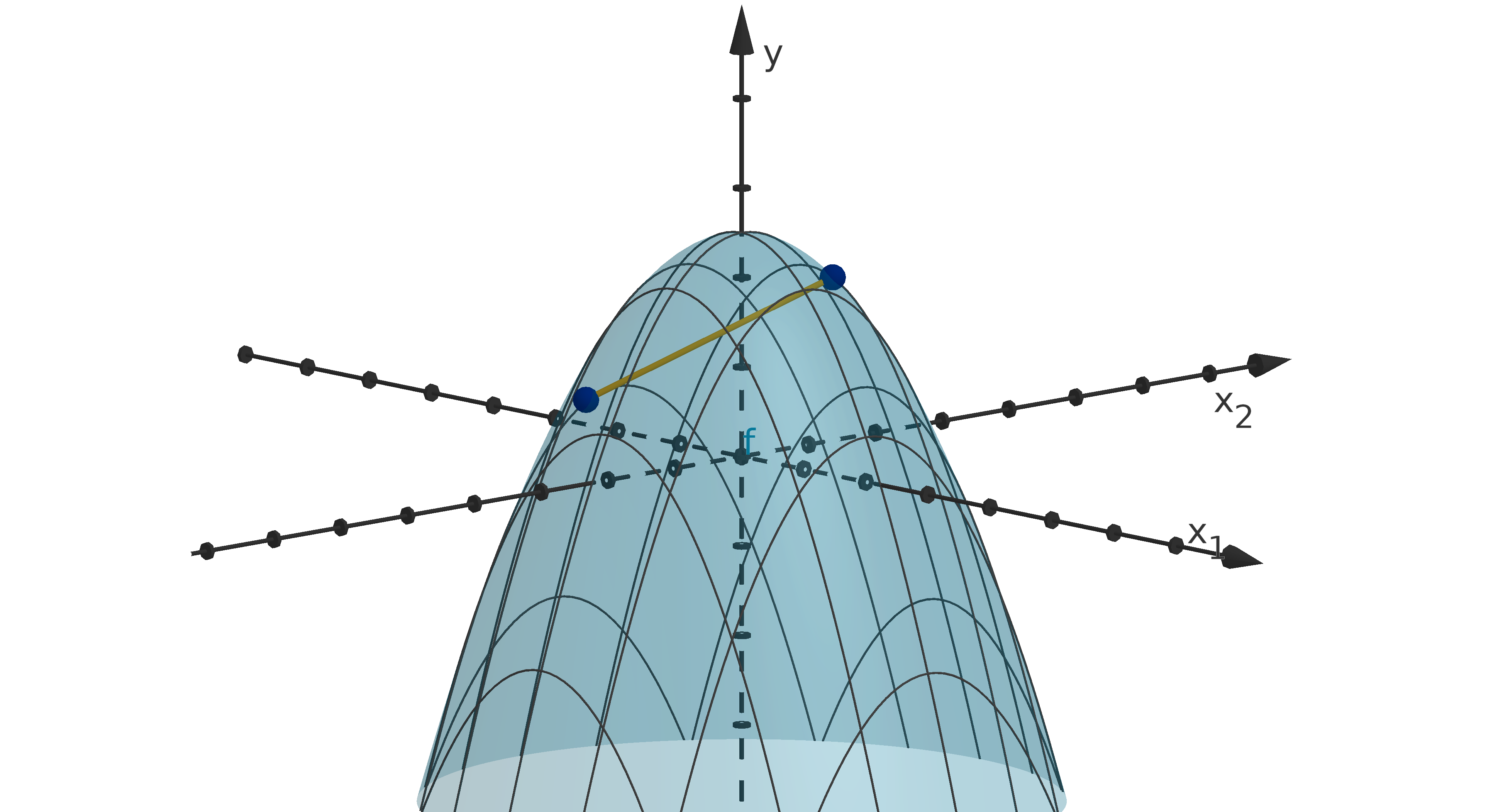
Figure 1.17: A secant below the graph of y = 5 − x

− x

We take two general points (a, f(a)) and (



b, f(



b)) on y = f(x). We parametrize the secant between

them.

x(t) =(1 − t)a + t



y(t) =(1 − t)f(a) + tf(



0 ≤ t ≤ 1

We can write an inequality to express the condition that secant lies below the graph.

Figure 1.18: A secant below the graph of a single-variable function

Theorem 1.19

A function is concave, if and only if for all a and



b in its domain and any 0 ≤ t ≤ 1 we have

(1 − t)f (a) + tf(



| {z }

height of secant

≤ f((1 − t)a + t



| {z }

height of y=f (x(t))

0 ≤ t ≤ 1

Remarks

This is an “if and only if” condition. That means it is both necessary and suﬃcient for establishing

concavity.

Only a function with a convex domain can meet this condition. Otherwise we cannot always

evaluate f((1 − t)a + t



b), because (1 − t)a + t



b may lie outside the domain.

The theorem follows directly from the deﬁnitions we have developed so far. Here is a representation

of our reasoning.

(1 − t)f(a) + tf(



b) ≤ f((1 − t)a + t



for all a,



b and t

The secant between any a and



lies under the graph y = f(x)

The region below y = f(x) is convex

f is concave

Applying the same reasoning to the deﬁnitions of convexity and strict concavity/convexity gives the

following variants. Note that we cannot demand a strict inequality at t = 0 or t = 1 because the secant

will always intersect the graph y = f(x) at a and b.

1.2.3 The Inequality Test for Concavity

Variants of Theorem 1.19

1 A function is convex, if and only if for all a and



b in its domain and any 0 ≤ t ≤ 1 we have

(1 − t)f (a) + tf(



b) ≥ f((1 − t)a + t



b) 0 ≤ t ≤ 1

2 A function is strictly concave, if and only if for all a and



b in its domain and any 0 < t < 1 we

have

(1 − t)f (a) + tf(



b) < f((1 − t)a + t



b) 0 < t < 1

3 A function is strictly convex, if and only if for all a and



b in its domain and any 0 < t < 1 we have

(1 − t)f (a) + tf(



b) > f((1 − t)a + t



b) 0 < t < 1

1.2.4

Verifying Concavity with an Inequality

Verify that f (x) = 5 − x

is concave using the inequality condition.

Solution

Let a and b be any two real numbers. We need to show that for all t in [0, 1]:

(1 − t)f (a) + tf(b) ≤ f((1 − t)a + tb)

To prove this inequality, we ﬁrst need the AM-GM (arithmetic mean-geometric mean) inequality from

algebra. Here it is.

(a − b)

≥ 0

− 2ab + b

≥ 0

+ b

≥ 2ab

We also note that for t in [0, 1], t(1 − t) ≥ 0. We now prove the required inequality, starting with

the right side.

f((1 − t)a + tb) = 5 − ((1 − t)a + tb)

deﬁnition of f

= 5 − (1 − t)

− 2t(1 − t)ab − t

distribute

≥ 5 − (1 − t)

− t(1 − t)(a

+ b

) − t

AM-GM

= 5 − (1 − t)

− t(1 − t)a

− t(1 − t)b

− t

distribute

= 5 − (1 − t)(t + 1 − t)a

− t(1 − t + t)b

factor

= 5 − (1 − t)a

− tb

simplify

= 5(1 − t) − (1 − t)a

+ 5t − tb

break up 5

= (1 − t)(5 − a

) + t(5 − b

) factor

= (1 − t)f (a) + tf(b) deﬁnition of f

The inequality condition is diﬃcult to verify, even for this simple function. It is much worse for a

function involving a square root or an exponential. On the other hand. The inequality condition can be

convenient for abstract results.

Theorem 1.20

If f(x) and g(x) are both concave, then so is their sum: h(x) = f(x) + g(x)

Proof

Let a and



b be in the domain of h. Since the domain of h is the intersections of the domains of f and g,

h has a convex domain (Theorem 1.15). We know from the concavity of f and g that for all t in [0, 1]:

(1 − t)f (a) + tf(



b) ≤ f((1 − t)a + t



(1 − t)g(a) + tg(



b) ≤ g((1 − t)a + t



We now verify that the inequality holds for h:

(1 − t)h(a) + th(



b) = (1 − t)f (a) + (1 − t)g(a) + tf(



b) + tg(



≤ f((1 − t)a + t



b) + g((1 − t)a + t



= h((1 − t)a + t



We conclude that h is concave.

1.2.4

Verifying Concavity with an Inequality

Main Idea

The inequality condition is sometimes useful at a theoretical level, but is painful to check for any but

the simplest speciﬁc functions. We will want a condition that is easier to check.

1.2.5

Concavity and Tangent Lines

We sought out the idea of concavity because it applies to functions of many variables. Some results

about concave functions are related to their derivatives. We will develop these tools in the setting

that is most comfortable and intuitive: one-variable functions. Once we have presented the theory of

optimization for multivariable functions, we will revisit and generalize these results.

Derivatives tell us about tangent lines, and tangent lines have an interesting relationship to convex

sets. If you draw a nonconvex set, you will be able to ﬁnd a tangent line that crosses through the set.

A convex set, on the other hand, lies entirely on one side of any of its tangent lines. We will not try

to prove this for general sets, but we will prove it for the strictly convex region below the graph of a

strictly concave function.

Lemma 1.21

If f(x) is a strictly concave function that is diﬀerentiable at a, then the rest of the graph y = f(x) lies

below its tangent line at (a, f(a)).

y = f(x)

Figure 1.19: The graph of a strictly concave function and some of its tangent lines

This lemma describes the relationship between y = f(x) and a single tangent line. It can apply to

a function that is not diﬀerentiable at other points in its domain. If the function is diﬀerentiable on its

entire domain, we can produce a necessary and suﬃcient condition on the tangent lines.

Theorem 1.22

Let f(x) be a diﬀerentiable function on a convex domain. f (x) is strictly concave, if and only if the

graph y = f(x) lies below all of its tangent lines (except at the point on tangency).

The proofs of these results are somewhat technical. We will provide them after we have discussed

applications.

1.2.6

Concavity Conditions for a Maximizer

Our main use of concavity (for now) is to produce suﬃcient conditions for maximizers. The following

corollary follows from Lemma 1.21.

Corollary 1.23

If f(x) is a strictly concave function and f

′

∗

) = 0, then x

∗

is the unique global maximizer of f.

Proof

The assumption that f

′

∗

) = 0 tells us that f is diﬀerentiable at x

∗

, and the tangent line at x

∗

horizontal. By Lemma 1.21, the rest of the graph lies below this line. We conclude that x

∗

is the unique

global maximizer.

y = f(x)

∗

, f(x

∗

))

Figure 1.20: The graph of y = f (x), which lies below the tangent line at x

∗

Like in the global second-order condition, we can also argue that x

∗

is the only critical point. If

there were another, then it would also be the unique global maximizer, which is nonsense.

1.2.7

A Second Derivative Test for Concavity

We would still like to have a better way to determine when a function is concave. In calculus, we

learn that the sign of the second derivative determines the concavity of a function. We are now in a

position to formally argue this result.

Theorem 1.24

If f is a function on a convex domain D ⊆ R and f

′′

(x) < 0 for all x in D, then f(x) is strictly

concave.

This means that a negative second derivative is a suﬃcient condition for strict concavity. Is it

necessary? No, consider the following.

Example

Consider f(x) = −x

. This function is strictly concave, but f

′′

(0) = 0, so the second derivative is not

always negative.

Putting this with Corollary 1.23 gives a string of conditions. Each is suﬃcient and neither is necessary,

so the implications can only be followed from left to right.

′′

(x) < 0

for all x

f strictly concave

Any x

∗

with f

′

∗

) = 0

is a maximizer

We could claim that Corollary 1.23 and Theorem 1.24 have combined to give an alternate argument

for the global second-order condition. However, proving Theorem 1.24 without the global second-order

condition would require us to redo much of the work that went into that theorem. Instead we will use

the global second-order condition to keep our proof of Theorem 1.24 brief.

Proof

Our goal is to apply Theorem 1.22. Let a be a point in the domain of f. Since f

′′

(x) exists, f

′

(a)

exists. Let y = ℓ(x) be the tangent line to y = f(x) at a. Let g(x) = f(x) − ℓ(x). We know the

following about g:

′′

(x) = f

′′

(x) − ℓ

′′

(x) < 0 for all x, since ℓ

′′

(x) = 0.

′

(a) = f

′

(a) − ℓ

′

(a) = 0, since the derivative is the slope of the tangent line.

g(a) = 0, since ℓ(a) = f(a).

g and a satisfy the conditions of the global second-order condition. Thus a is the unique maximizer of

g, meaning g(x) < g(a) = 0 for all x = a. Thus y = f (x) lies below y = ℓ(x). This reasoning holds for

the tangent line at any value a. Theorem 1.22 tells us that f is strictly concave.

y = f(x)

y = g(x)

(a, f(a))

Figure 1.21: The graph of f(x), the tangent line at a, and their diﬀerence

1.2.8

Verifying Concavity with the Second Derivative

Verify that f (x) = 5 − e

is strictly concave.

Solution

′′

(x) = −e

< 0 for all x. Therefore by Theorem 1.24, f (x) is strictly concave.

Main Idea

The second derivative is an easier test of strict concavity than the inequality we used earlier, but it is

only a suﬃcient condition. It does not detect every strictly concave function.

1.2.9

Proving the Relationship Between Concavity and Tangent Lines

We will now present the formal reasoning of Lemma 1.21 and Theorem 1.22. We prove Lemma 1.21

by examining the diﬀerence between f(x) and its secants.

1.2.9 Proving the Relationship Between Concavity and Tangent Lines

Proof

Pick any b = a on the graph y = f (x). The tangent line to y = f (x) at (a, f (a)) has equation

y = f(a) + f

′

(a)(x −a). We will ﬁrst show that (b, f(b)) does not lie above the tangent line by showing

that f(b) ≤ f(a) + f

′

(a)(b − a).

Consider the case that b > a. Denote the secant from (a, f(a)) to (b, f(b)) by the equation y = s(x)

and let g(x) = s(x) − f(x). The region below y = f(x) is convex, so y = s(x) is below y = f(x)

for any x between a and b. Their diﬀerence, g(x), is less than or equal to 0 on this interval. By the

contrapositive of Lemma 1.2 we know g

′

(a) cannot be greater than 0.

′

(a) is the slope of the secant:

f(b) − f(a)

b − a

. We substitute this into g

′

(a) ≤ 0 and solve.

′

(a) ≤ 0

′

(a) − f

′

(a) ≤ 0 (sum rule)

f(b) − f(a)

b − a

− f

′

(a) ≤ 0 (substitute)

f(b) − f(a) − f

′

(a)(b − a) ≤ 0 (b − a > 0)

f(b) ≤ f(a) + f

′

(a)(b − a)

We conclude that (b, f(b)) does not lie above the tangent line.

Now we must also show it does not lie on the tangent line. This is easiest with a contradiction

argument. Suppose some (b, f(b)) lies on the tangent line at a. Then consider any c between a and b.

(c, f(c)) also does not lie above tangent line by the argument we gave for b. However, the secant from

(a, f(a)) to (b, f(b)) is part of the tangent line, and (c, f(c)) lies above this by the deﬁnition of strict

concavity. This is a contradiction. Thus there is no (b, f(b)) that lies on the tangent line.

The case where b < a can be proved with a similar argument. We conclude that (b, f(b)) lies below

the tangent line to y = f(x) at (a, f(a)).

y = f(x)

y = s(x)

(a, f(a))

(b, f(b))

Figure 1.22: A tangent line and a secant to a concave function

Theorem 1.22 is an “if and only if” statement, so it requires two arguments to prove. We must

show that if f is strictly concave, then its graph lies below its tangent lines. We must also show that if

its graph lies below its tangent lines, then it is strictly concave. Fortunately, Lemma 1.21 has already

shown that if f (x) is strictly concave, then y = f(x) lies below the tangent line at a.

Proof

Suppose we know f is concave. For each a in the domain of f, Lemma 1.21 states that y = f (x) lies

below its tangent line at a. Since this holds for all a, y = f(x) lies below all of its tangent lines.

Now suppose that we know y = f (x) lies below all its tangent lines. We will verify that the region

under y = f (x) is strictly convex. Let a and b be any points in the domain of f . Let c be any point

between them. We know that (a, f(a)) and (b, f(b)) both lie below the tangent line to y = f(x) at

(c, f(c)). Thus the tangent line lies above the entire secant between (a, f(a)) and (b, f(b)). (c, f(c))

is on this tangent line, so (c, f(c)) is above the secant as well.

Since this argument holds for any such c, we conclude that the entire graph between a and b lies

above the secant. Since this is true for any choice of a and b, we conclude that the region below

y = f(x) is strictly convex and f (x) is a strictly concave function.

y = f(x)

(a, f(a))

(c, f(c))

(b, f(b))

Figure 1.23: A secant with both endpoints below the tangent line at (c, f(c))

1.2.10

Non-Strict Concavity and Convexity

We have primarily worked with strictly concave functions, because they give the strongest results

about maximizers. The properties of non-strict concavity and convexity give similar results. The results

for convexity are obtained by ﬂipping the directions of inequalities. They are probably not worth mem-

orizing. On the other hand, economists frequently need to work with non-strictly concave functions. It

is worth understanding how utility maximization works for these.

Graphs of non-strictly concave functions can intersect their own tangent lines. For instance, a linear

function is concave, and its graph is identical to its tangent line. While the graph of a concave function

can intersect the tangent lines, it cannot go above them.

1.2.10 Non-Strict Concavity and Convexity

Variants of Lemma 1.21

Let f(x) be a function on a convex domain.

1 If f (x) is a concave function that is diﬀerentiable at a, then the graph y = f(x) has no points

above its tangent line at (a, f(a)).

2 If f(x) is a strictly convex function that is diﬀerentiable at a, then the rest of the graph y = f (x)

lies above its tangent line at (a, f(a)).

3 If f(x) is a convex function that is diﬀerentiable at a, then the graph y = f(x) has no points

below its tangent line at (a, f(a)).

The proof for non-strict concavity is identical to the proof for strict concavity, with the contradiction

argument omitted. The necessary and suﬃcient conditions are unsurprising.

Variants of Theorem 1.22

Let f(x) be a diﬀerentiable function on a convex domain.

1 f(x) is concave if and only if the graph y = f(x) has no points above any of its tangent lines.

2 f(x) is strictly convex if and only if the graph y = f(x) lies above each of its tangent lines (except

at the point of tangency).

3 f(x) is convex if and only if the graph y = f(x) has no points below any of its tangent lines.

These results can also be extended to well-behaved non-diﬀerentiable functions. For instance, what-

ever “tangent lines” you might reasonably add to the function in Figure 1.16 will not stray below the

graph. Rigorously deﬁning tangent lines in these situations would require a detailed argument involving

limits, so we will not pursue it here.

The variants of Lemma 1.21 give rise to their own corollaries about maximizers and minimizers.

Variants of Corollary 1.23

1 If f(x) is a concave function and f

′

∗

) = 0, then x

∗

is a global maximizer (but other points may

be as well).

2 If f(x) is a strictly convex function and f

′

∗

) = 0, then x

∗

is the unique global minimizer of f.

3 If f(x) is a convex function and f

′

∗

) = 0, then x

∗

is a global minimizer (but other points may

be as well).

∗

, f(x

∗

))

Figure 1.24: A global but non-unique maximizer of a not strictly concave function

Finally, we can use the Variants of Theorem 1.22 to produce second-derivative tests for the other

forms of concavity and convexity.

Variants of Theorem 1.24

1 If f is a function on a convex domain D ⊂ R and f

′′

(x) ≤ 0 for all x in D, then f(x) is concave.

2 If f is a function on a convex domain D ⊂ R and f

′′

(x) > 0 for all x in D, then f(x) is strictly

convex.

3 If f is a function on a convex domain D ⊂ R and f

′′

(x) ≥ 0 for all x in D, then f(x) is convex.

In the non-strict case, the condition is necessary as well as suﬃcient.

1.2.10 Non-Strict Concavity and Convexity

Corollary 1.25

A twice diﬀerentiable function f(x) on a convex domain D is concave, if and only if f

′′

(x) ≤ 0 for all

x in D.

The suﬃciency of f

′′

(x) ≤ 0 is found in the preceding variant. We establish necessity with a

contrapositive argument. It should look familiar to anyone who read our proof of Theorem 1.24. Notice

that it is making a local rather than a global argument.

Proof

Suppose f

′′

(x) ≤ 0 for all x. A variant of Theorem 1.24 tells us that f is concave.

On the other hand, suppose f

′′

(a) > 0 for some a. First note than since f

′′

(x) exists, f is a

diﬀerentiable function. Let y = ℓ(x) be the tangent line to y = f(x) at a. Consider g(x) = f(x)−ℓ(x).

We know the following about g:

′′

(a) = f

′′

(a) − ℓ

′′

(a) > 0, since ℓ

′′

(x) = 0.

′

(a) = f

′

(a) − ℓ

′

(a) = 0, since the derivative is the slope of the tangent line.

g(a) = 0, since f(a) = ℓ(a).

Thus by a variant of the (local) second-order condition, Theorem 1.5, a is a strict local minimizer of g,

meaning g(x) > g(a) = 0 for all x in a neighborhood of a. Thus y = f(x) lies above y = ℓ(x) in this

neighborhood. By a variant of Theorem 1.22, f is not concave.

The contrapositive of this argument is that if f is concave, then there is no a such that f

′′

(a) > 0.

Equivalently, f

′′

(x) ≤ 0 for all x.

This result means that we not only have a way to show that f(x) is concave, but also that it is not

concave. If f

′′

(a) > 0 for any a, then f is not a concave function.

1.2.11

Section Summary

The most important deﬁnitions and results from this section were

The deﬁnition of a (strictly) convex region (Deﬁnitions 1.12 and 1.14)

The deﬁnition of a (strictly) concave function (Deﬁnitions 1.16 and 1.17)

The inequality condition for concave functions (Theorem 1.19)

The tangent line condition for strictly concave functions (Theorem 1.22)

The suﬃcient condition for a maximizer using strict concavity (Corollary 1.23)

The second derivative tests for strictly concave and concave functions (Theorem 1.24 and Corollary

1.25)

Here is a summary of which conditions and statements from this section imply which others. Some

of these conditions only apply to diﬀerentiable, or even twice diﬀerentiable functions.

If f diﬀerentiable

(twice if relevant)

(1 − t)f (a) + tf(b) < f((1 − t)a + tb) (1 − t)f (a) + tf(b) ≤ f((1 − t)a + tb)

f strictly concave f concave

y = f(x) below tangent lines y = f(x) not above tangent lines

′′

(x) < 0 f

′′

(x) ≤ 0

critical points are unique maximizers critical points are maximizers

Figure 1.25: Conditions and applications of concave functions

1.3

Multivariable Optimization

Goals:

1 Apply the ﬁrst- and second-order conditions to multivariable functions

2 Calculate the Hessian of a function

3 Understand the deﬁnition and signiﬁcance of positive or negative deﬁnite matrices

4 Test whether a matrix is positive or negative deﬁnite

5 Show that a multivariable function is strictly concave

1.3.1

Parametrizations and Compositions

In this section we develop conditions to ﬁnd maximizers of multivariable functions. Our optimization

methods so far rely on using rates of change to compare a potential maximizer to the points around it.

This is a more daunting task in the multivariable situation, because the comparison points can lie in any

direction. The function can be changing diﬀerently depending on which direction we travel. We avoid

the need to develop now tools from scratch by considering paths through a potential maximizer a.

A path through a is a function x(t) such that for some t

, x(t

) = a. We can think of the variable

t as representing time. Then x(t) represents the position on our path at time t.

A path breaks down into coordinate functions

x(t) = (x

(t), x

(t), . . . , x

(t))

If these are diﬀerentiable, the derivative

x

′

(t) = (x

′

(t), x

′

(t), . . . , x

′

(t))

represents the instantaneous rate of change in position of x with respect to t. It is tangent to the

path. In physics it is called the velocity vector.

Figure 1.26: A path and its tangent vector

We will study a function f(x) by studying compositions of the form f (x(t)). At each value of t, we

compute the corresponding position on the path and then evaluate f at that position. Geometrically,

this is the height of the graph y = f(x) above the curve x(t).

Figure 1.27: The graph of the composition f(x(t)) and the corresponding points in the original graph

y = f(x)

The derivative of f(x(t)) with respect to t is computed using the multivariable chain rule.

1.3.1

Parametrizations and Compositions

Theorem 0.18

Suppose f(x) is an continuously diﬀerentiable n-variable function. If x(t) is a diﬀerentiable path, then

the derivative of the composition f(x(t)) with respect to t is

(t) = ∇f(x(t)) · x

′

(t)

(t) =

i=1

(x(t))x

′

(t)

As with single-variable optimization, the sign of a derivative is important to our arguments. We can

obtain the sign of

visually, using the following fact about dot products.

The Sign of the Dot Product

Given nonzero vectors u and v, the sign of u ·v is

positive if u and v make an acute angle

zero if u and v are orthogonal

negative if u and v make an obtuse angle

The angle between ∇f and x

′

(t) determines the sign of

. This indicates whether f(x) increases

or decreases as x travels along the path x(t).

Figure 1.28: The tangent line to the graph y = f (x(t)) and the angle between ∇f (x(t)) and x

′

(t)

The value of

is realized geometrically as the slope of the tangent line to the graph of the

composition function: y = f (x(t)).

Using compositions to ﬁnd maximizers has two main consequences. The ﬁrst is helpful. The second

creates diﬃculties.

1 f(x(t)) is a one-variable function. No matter the dimension of x, we can graph y = f(x(t)) in

the ty-plane and look for maximizers there.

2 One path will not cover the whole domain of f(x). We have to study many diﬀerent paths x(t),

if we want to compare a potential maximizer to every other point in the domain.

We could study all paths in the domain of f, but that would be needlessly diﬃcult. Instead we

restrict ourselves to paths that are lines. We will express these lines using the following notation.

Notation

Every line has a direction vector v = (v

, v

, . . . , v

). A line through a in the direction of v has the

equation

x(t) = a + tv

In a convex domain, any two values f (a) and f(



b) can be attained as values of the composition

f(a + tv), where v =



b −a. If we want to compare these values (for instance to argue that a is or is

not a maximizer), we compare f(a + 0v) and f (a + 1v).

Lemma 1.26

Suppose f (x) has a convex domain. A point a is a (local or global) maximizer, if and only if 0 is a

(local or global) maximizer of f(a + tv) for all direction vectors v.

This lemma tells us that a necessary condition for 0 to be a maximizer of f(a + tv) for all v is

a necessary condition for a to be a maximizer of f(x). Similarly, a suﬃcient condition for 0 to be a

maximizer of f(a + tv) for all v is a suﬃcient condition for a to be a maximizer of f(x).

The compositions f(a + tv) are realized as cross sections of the graph y = f(x) above the line

x(t) = a + tv.

1.3.1

Parametrizations and Compositions

Figure 1.29: The graph of a two-variable function and its cross section over a line

1.3.2

The Multivariable First-Order Condition

Our starting point for multivariable optimization is Lemma 1.26. a is a local maximizer or minimizer

of f (x), if and only if 0 is a local maximizer or minimizer of f(a + tv) for all vectors v. A condition on

the compositions f(a + tv) at t = 0 becomes a condition on a.

The ﬁrst-order condition on f(a + tv) at t = 0 is

(0) = 0

∇f(a + 0v) ·v = 0

∇f(a) ·v = 0

If a is a local maximizer, this must hold for all directions v. There is only one value of ∇f(a) that

satisﬁes this requirement.

Theorem 1.27 [The Multivariable First-Order Condition]

Suppose a lies in the domain of f (x). If a is a local maximizer or minimizer of f, then either ∇f(a) =



or ∇f (a) does not exist.

Like in the single variable case, we call points where ∇f (x) is



0 or undeﬁned critical points. Finding

critical points is often the ﬁrst step in a multivariable optimization.

Remark

If a lies at the boundary of the domain, then it may not be possible to travel in all directions v from

a and still evaluate f(a + tv). Fortunately, the ﬁrst-order condition still holds. If ∇f(a) exists, then

the partial derivatives f

(a) exist. Thus f (a + he

) exists for h near 0. That means we can at least

travel in the standard basis directions from a without immediately leaving the domain of f(x). At a

local maximizer, the derivatives in these directions must be 0.

1.3.3

Computing Critical Points

What does the multivariable ﬁrst-order condition say about f (x

, x

) = x

− 4x

+ x

Solution

We compute the gradient vector by taking the partial derivatvies with respect to x

and x

∇f(x) = (f

(x), f

(x))

= (4x

− 4x

, 4x

+ 4x

)

This is never undeﬁned, so we solve for where it is (0, 0).

− 4x

= 0 −4x

+ 4x

= 0

= x

(solve for x

)

−4x

+ 4x

= 0 (substitute)

− 1) = 0 (factor)

= 0 or ± 1

Subsituting back into x

= x

gives lets us solve for the corresponding values of x

. We obtain the

critical points (0, 0), (1, 1) (−1, −1). We conclude that no point other than (0, 0), (1, 1) (−1, −1) can

be a local maximizer or a local minimizer. We cannot conclude whether each of these points is a local

maximizer, a local minimzer or neither.

1.3.4

The Second Derivative of a Composition

We would also like to apply the local or global second-order condition along each line. In order to

do this, we need a way to compute

f(a + tv). The chain rules allows us to write the ﬁrst derivative

as a dot product, or a sum. We will write it as a sum.

f(a + tv) =

i=1

(a + tv)v

To obtain the second derivative we diﬀerentiate both sides. We diﬀerentiate each term of the sum. We

can treat each v

as a constant multiple, but f

(a + tv) is a composition of functions. The derivative

of each term will need the chain rule. We again write this as a sum, using a diﬀerent index variable to

avoid ambiguity. The partial derivatives of f

are f

f(a + tv) =

i=1

(a + tv)v

f(a + tv) =

i=1

(a + tv)) v

f(a + tv) =

i=1





j=1

(a + tv)v





f(a + tv) =

i=1

j=1

(a + tv)v

We could use this formula to compute the second derivative of a particular composition f(a + tv). We

could test whether it is positive or negative. What we need, though, is to test the sign of the second

derivative for all direction vectors v. While this is possible in small dimensions, leaving the v

as variables,

the algebra quickly becomes daunting as n increases.

1.3.5

The Hessian Matrix

A theorem in linear algebra provides a shortcut. To do linear algebra, we need to write our vectors

like matrices.

Point Form and Column Form

When we want to emphasize that a vector x represents a point in R

, we write it as x = (x

, x

, . . . x

If we want to do matrix multiplication, we can write it as a column vector:

x =













The expression

f(a + tv) =

i=1

j=1

(a + tv)v

that we obtained can be written as a matrix product.

··· v







(a + tv) f

(a + tv) ··· f

(a + tv)

(a + tv) f

(a + tv) ··· f

(a + tv)

(a + tv) f

(a + tv) ··· f

(a + tv)



















You may want to convince yourself that this algebra is correct with a 2 or 3 dimensional example.

What do we make of the individual factors in this product? The vectors on either end of this expression

are just v and its transpose (v ﬂipped sideways). The matrix in the middle seems important. We should

have a name for it.

Deﬁnition 1.28

Given a function f(x) of n variables, the Hessian is a n ×n matrix function of x whose entries are the

second partial derivatives of f at x. Its formula is

Hf (x) =







(x) f

(x) ··· f

(x)

(x) f

(x) ··· f

(x)

(x) f

(x) ··· f

(x)







Notice that for well-behaved functions, f

= f

. This means the Hessian will be a symmetric

matrix.

1.3.6

Negative Deﬁnite Matrices

Our Hessian notation allows us to write

f(a + tv) = v

Hf (a + tv)v. The following vocabulary

captures exactly which Hessian matrices will produce a negative (or positive) second derivative in all

directions.

Deﬁnition 1.29

A symmetric n × n matrix M is negative deﬁnite, if for all nonzero n-vectors v,

v

Mv < 0.

It is positive deﬁnite, if for all nonzero n-vectors v,

v

Mv > 0.

Remark

We may think, based on positive and negative numbers, that most matrices are either positive deﬁnite

or negative deﬁnite. In fact, a randomly chosen matrix is most likely to be neither. For most matrices,

v

Mv is positive for some v and negative for others.

Connecting this back to our original goal, we can apply the deﬁnition of negative deﬁnite to describe

the sign of the second derivatives of the compositions f(a + tv). For a critical point a, we can draw the

following conclusions.

If Hf(a) is negative deﬁnite, then

(0) < 0 for all v. Since

(0) = 0, t = 0 satisﬁes the

second-order condition for all v. We conclude a is a strict local maximizer of f.

If Hf (x) is negative deﬁnite for all x, then

(t) < 0 for all t and all v. Since

(0) = 0, t = 0

satisﬁes the global second-order condition for all v. We conclude a is the unique global maximizer

of f.

Without an eﬃcient way to test whether a matrix is negative deﬁnite, we have only managed to

restate the problem. We can say that we are checking whether Hf(a) is negative deﬁnite, or we can

say that we are checking whether

i=1

j=1

(a)v

< 0 for all v

, v

, . . . , v

. The computations are

the same, and they are daunting.

Fortunately, there is an easier way to show that a matrix is negative or positive deﬁnite.

Theorem 1.30

A symmetric n ×n matrix M is negative deﬁnite if the upper left square minors M

have determinants

that satisfy the alternating condition:

(−1)

| > 0 for all 1 ≤ i ≤ n

Example

For a 4 × 4 matrix, here are the M

and what we would check to apply Theorem 1.30.







· · · ·







| < 0

| > 0

| < 0

| > 0

Variant of Theorem 1.30

A n × n matrix M is positive deﬁnite if the upper left square minors have positive determinants.

1.3.7

The Multivariable Second-Order Conditions

Now that we have a check for negative deﬁnite and positive deﬁnite matrices, it is worth stating

the results of our investigation as theorems. These are our most important suﬃcient conditions for a

maximizer of a multi-variable function.

1.3.7 The Multivariable Second-Order Conditions

Theorem 1.31 [The Multivariable Second-Order Condition]

Given a function f(x) with a it its domain. If

∇f(a) =



Hf (a) is negative deﬁnite

then a is a strict local maximizer of f.

Theorem 1.32 [The Multivariable Global Second-Order Condition]

Suppose f is a function with a convex domain D and x

∗

is in D. If

∇f(x

∗

) =



Hf (x) is negative deﬁnite for all x ∈ D.

then x

∗

is the only critical point of f and the unique global maximizer.

We can summarize the reasoning behind the global second-order condition as follows:

Hf (x) is negative deﬁnite

for all x

f(x

∗

+ tv) < 0 for

all directions v

∇f(x

∗

) =



(0) = 0 along

all lines x

∗

+ tv

0 is the global maximizer

of f(x

∗

+ tv) for all directions v

x

∗

is the global maximizer of f(x)

These theorems have variants for minimizers.

Variants of Theorems 1.31 and 1.32

Suppose f is a function with domain D and a is in D.

1 If

∇f(a) =



Hf (a) is positive deﬁnite

then a is a strict local minimizer of f.

2 If D is convex and

∇f(a) =



Hf (x) is positive deﬁnite for all x in D

then a is the only critical point of f and the unique global minimizer.

Minor determinants with the wrong sign produce the wrong sign of v

Mv for some v. This in turn

means the wrong second derivative in the direction of v. This relationship is formalized in the following

necessary condition.

Corollary 1.33

Let f(x) be a twice-diﬀerentiable function on a convex domain D. Let M = Hf(a).

1 If a is a local maximizer, then

(−1)

| ≥ 0 for all 1 ≤ i ≤ n.

2 If a is local minimizer, then

| ≥ 0 for all 1 ≤ i ≤ n.

1.3.8

Applying the Multivariable Second-Order Condition

Let f(x

, x

) = 3

√

+ln x

−

−2x

+15 on the domain D = {(x

, x

) : x

, x

0}. Find the critical point of f. What does the Global Second-Order Condition say about this point?

1.3.8

Applying the Multivariable Second-Order Condition

Solution

We take all three partial derivatives of f. Since they are always deﬁned on D, the gradient vector exists,

so the critical points must be where they all equal 0.

√

−

= 0

−

= 0

√

− 2 = 0

√

= 2

√

= 5

√

= 2

8 = x

√

= 1

The critical point is (8, 5, 1). We compute the Hessian by taking the second partial derivatives of f .

Hf (x

, x

) =







−

√

0 −

√

0 −

√







To check that Hf(x) is negative deﬁnite for all x, we apply Theorem 1.30. There are three determinants

to calculate.

(−1)

| = (−1)



−

√



√

(−1)

| = (1)



−

√

0 −



√

(−1)

| = −|Hf(x

, x

= −

−

√



−

0 −

√



− 0 +



0 −

√



−

Since x

, x

and x

are all positive in this domain, so are these three quantities. We conclude that

Hf (x

, x

) is negative deﬁnite. By the global second-order condition, we conclude that (8, 5, 1) is

the only critical point (which we already knew from the FOC) and that it is the unique maximizer of f .

1.3.9

The Hessian and Concavity

Linear compositions play well with secants. The height of the secant above each t is the same

whether we are looking in ty-plane or in R

n+1

. We can state this relationship formally as a lemma.

Lemma 1.34

If y = s(t) is a secant of y = f (a + tv), then

x(t) = a + tv

y(t) = s(t)

is a secant of y = f(x).

Figure 1.30: A secant of y = f (a + tv) and the corresponding secant of y = f(x) over x(t) = a + tv

We determine whether a function f(x) is concave by whether its graph lies above its secant lines.

Every such secant line lies above some line a + tv. This secant stays below the graph y = f(x), if and

only if the corresponding secant stays below y = f(a + tv).

1.3.9 The Hessian and Concavity

Lemma 1.35

A function f(x) on a convex domain is concave, if and only if f(a + tv) is concave for every a in the

domain of f and every direction vector v.

f(a + tv) is concave

for all lines a + tv

y = f(a + tv) lies above

its secants (t, s(t))

for all lines a + tv

y = f(x) lies above the secants

x(t) = a + tv

y(t) = s(t)

for all lines a + tv

f(x) is concave

Def 1.16

Cor 1.34

Def 1.16

Variants of Lemma 1.35

Suppose f(x) is a function on a convex domain

1 f(x) is strictly concave if and only if f(x(t)) is strictly concave for every line x(t) in the domain

of f.

2 f(x) is convex if and only if f (x(t)) is convex for every line x(t) in the domain of f.

3 f(x) is strictly convex if and only if f(x(t)) is strictly convex for every line x(t) in the domain of

The result of this lemma is that any test for concavity or convexity of the single-variable compositions

f(a + tv) becomes a test for the concavity of f(x) itself. If every composition passes, then f does.

If at least one composition fails, then so does f. Our natural next step is to take our theorems from

single-variable concavity and apply them to these compositions,

Theorem 1.22 showed that the graphs single-variable strictly concave functions lie below their tangent

lines. Tangent lines to a composition have the same heights as the tangent lines of the multivariable

graph. We can formalize this relationship with a lemma.

Lemma 1.36

If the line y = ℓ(t) is tangent to y = f (a + tv), then

x(t) = a + tv

y(t) = ℓ(t)

is a tangent line to y = f(x).

Figure 1.31: A tangent line of y = f (a + tv) and the corresponding tangent line of y = f(x) over

x(t) = a + tv

We can check whether tangent lines lie above or below a graph y = f(x) by checking whether

tangent lines lie above or below the compositions y = f(a + tv).

Theorem 1.37 [Multivariable version of Theorem 1.22]

A diﬀerentiable function f on a convex domain is strictly concave if and only if the graph y = f(x) lies

below each of its tangent lines (except at the point of tangency).

y = f(x) lies below

its tangent lines.

y = f(a + tv) lies below all

its tangent lines for any a + tv.

f(a + tv) is strictly concave

for any a + tv

f(x) is strictly concave

Cor 1.36

Thm 1.22

Lem 1.35

This theorem allows us to update our corollary on critical points of strictly concave functions.

Corollary 1.38 [Multivariable Version of Corollary 1.23]

If x

∗

is a critical point of a diﬀerentiable, strictly concave function f(x), then it is the only critical

point and is the unique global maximizer.

1.3.9 The Hessian and Concavity

We can also use compositions to update our theorems about second derivatives and concavity.

Theorem 1.39 [Multivariable Version of Theorem 1.24]

If f is a function on a convex domain D ⊂ R

and

f(a + tv) < 0 for all lines a + tv in D, then

f(x) is strictly concave.

Corollary 1.40 [Multivariable Version of Corollary 1.25]

A twice diﬀerentiable function f(x) on a convex domain D is concave, if and only if

f(a + tv) ≤ 0

on all lines a + tv in D.

As we have seen, the sign of these second derivatives depends on the Hessian matrix. This gives us

our most useful computational test for the concavity of a multivariable function.

Theorem 1.41

Let f(x) be a twice-diﬀerentiable function on a convex domain D. If Hf (x) is negative deﬁnite for all

x in D, then f is strictly concave.

This means that concavity plays the same role in multivariable optimization as in single-variable

optimization. For some functions, we can identify a maximizer by concavity even though they do not

satisfy the second-order condition. On the other hand, the most convenient way to identify concave

functions is still the second derivatives.

1.3.10

Negative Semi-Deﬁnite Matrices

Changing the condition f

′′

(x) < 0 to f

′′

(x) ≤ 0 was a natural approach to generalizing Theorem

1.24. As a bonus, we obtained Corollary 1.25, which is both a necessary and suﬃcient condition

for concavity. The same is possible for multivariable functions, but the condition on the Hessian is

surprisingly complicated.

We might expect the multivariable analogue to be that (−1)

| ≥ 0 for each i. Consider a

function like f(x

, x

) = x

. In the x

direction this function is a parabola which is strictly convex.

Unfortunately, its Hessian passes our expected test for concavity.

Hf (x

, x

) =





0 0 0

0 0 2





This has |M

| = 0 for each i. The determinant cannot detect the curvature of later variables, if the

earlier variables produce a row of zeroes in Hf(x). Our expected test is not a correct test. To avoid

this problem, we must consider diﬀerent orders of variables. Which orders? All of them.

Theorem 1.42

Let f(x) be a twice-diﬀerentiable function on a convex domain D ⊆ R

. let σ be any reordering of

the coordinates of R

. Let σM = Hf(σx).

1 f is concave if and only if

(−1)

|σM

| ≥ 0 for all σ and all 1 ≤ i ≤ n.

If so, then v

Hf (x)v ≤ 0 for all nonzero v. We say Hf(x) is negative semideﬁnite

2 f is convex if and only if

|σM

| ≥ 0 for all σ and all 1 ≤ i ≤ n.

If so, then v

Hf (x)v ≥ 0 for all nonzero v. We say Hf(x) is positive semideﬁnite

To give a sense of the amount of computation required, we will consider an example. Suppose

Hf (x) =





0 2 5

2 −6 0

5 0 −3





We check the determinants

| = |0| ≤ 0 |M

| =



0 2

2 −6



≥ 0 |M

| =



0 2 5

2 −6 0

5 0 −3



≤ 0

1.3.10 Negative Semi-Deﬁnite Matrices

But then we must do the same for all possible reorderings of x

, x

and x

meaning we must check

the same three minors for each of





0 2 5

2 −6 0

5 0 −3





original Hf(x)





−6 2 0

2 0 5

0 5 −3





σ switches x

and x





−3 0 5

0 −6 2

5 2 0





σ switches x

and x





0 5 2

5 −3 0

2 0 −6





σ switches x

and x





−6 0 2

0 −3 5

2 5 0





σ : (x

, x

) 7→ (x

, x

)





−3 5 0

5 0 2

0 2 −6





σ : (x

, x

) 7→ (x

, x

)

This is a signiﬁcant amount of work, though linear algebra knowledge lets us avoid some. For

instance, all the |σM

| are equal. As the dimension increases, there are more symmetries to exploit.

With these shortcuts, the main driver in complexity is computing the n×n determinant, not the number

of re-ordered smaller determinants. Checking whether a matrix is negative semideﬁnite takes about twice

as many operations as checking that it is negative deﬁnite.

1.3.11

Section Summary

The most important deﬁnitions and results from this section were

The multivariable ﬁrst-order condition (Theorem 1.27)

The Hessian matrix (Deﬁnition 1.28)

Positive and negative deﬁnite (Deﬁnition 1.29)

The determinant test for a negative deﬁnite matrix (Theorem 1.30)

The multivariable global second-order condition (Theorem 1.32)

The Hessian test for strict concavity (Theorem 1.41)

Here is a summary of which conditions and statements from this section imply which others.

Hf (x) negative

deﬁnite for all x

Hf (x) negative semi-

deﬁnite for all x

Hf (a) negative

deﬁnite

f is strictly concave

f is concave

a is the

unique global max

and only critical point

a is a

global max

a is a strict

local max

∇f(a) =



∇f(a) =



Hf (a) negative

semideﬁnite

Thm 1.41

Thm 1.42

SOC

GSOC

FOC

Thm 1.33

Figure 1.32: Relationships between the conditions of multivariable optimization

1.3.11

Section Summary

Chapter 2

Constrained Optimization

2.1

Equality Constraints

Goals:

1 Use logic to reason about the eﬀects of a constraint on optimization problems.

2 Visually identify maximizers and minimizers using level sets.

3 Compute the maximizer subject to an equality constraint using the Lagrangian.

4 Use paths and the chain rule to understand the reasoning behind the Lagrangian.

2.1.1

Constrained Optimization

Given a function f (x) with domain D, we have so far performed unconstrained optimization, trying

to compute

max

x∈D

f(x) or min

x∈D

f(x)

In a constrained optimization problem, we restrict our attention to a subset of the domain. For some

subset S ⊆ D, we want to know

max

x∈S

f(x) or min

x∈S

f(x)

A maximizer in S is a vector a such that f(a) ≥ f(x) for all x ∈ S. Geometrically, it is the highest

point on the part of the graph y = f(x) that lies above S. In constrained optimization, the function we

are maximizing is called a objective function. The set S is called the feasible set.

The notation above is ﬂexible enough to apply to many diﬀerent kinds of constraints, producing

many diﬀerent kinds of subset S.

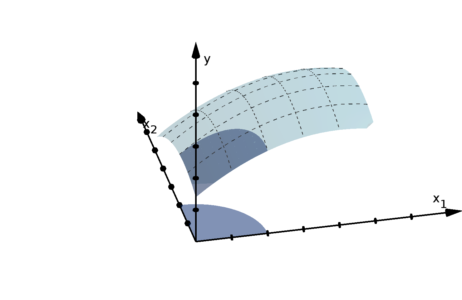
Figure 2.1: The graph y = f (x) over a two-dimensional subregion S

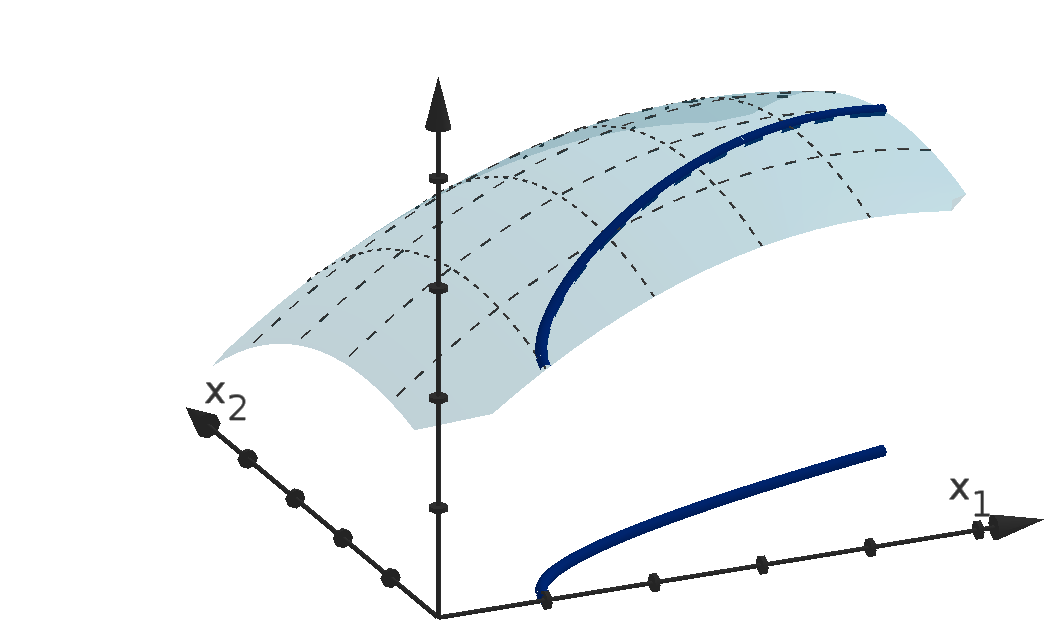
Figure 2.2: The graph y = f (x) over a curve S

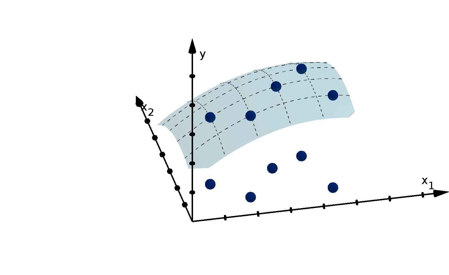
Figure 2.3: The graph y = f (x) over a ﬁnite set S

Constraints arise naturally in economics. Here are two familiar examples recast in the abstract form

that we just introduced.

Example

What is the maximum utility one can attain given a budget constraint?

max

x∈S

u(x)

where S is the set of purchases one can aﬀord.

2.1.1

Constrained Optimization

Example

How cheaply can a ﬁrm produce 500 units?

min

x∈S

c(x)

Here, S is the set of inputs that produce 500 units.

Without knowing the speciﬁc nature of the constraint, we can still deduce some basic facts about

constrained optimization using logic and set theory.

Tightening a constraint can only reduce the value of the maximum.

Lemma 2.1

For a function f(x) with domain D and a two subsets T ⊆ S ⊆ D,

max

x∈T

f(x) ≤ max

x∈S

f(x)

Sometimes ﬁnding a maximum over S is computationally easier than ﬁnding a maximum over T . If

we are lucky, the maximizer of f(x) in S might also lie in T . We can apply the following reasoning.

Corollary 2.2

Suppose x

∗

is a maximizer of f(x) over a set S. If T ⊆ S and x

∗

∈ T then x

∗

is also a maximizer of

f(x) over T and

max

x∈T

f(x) = max

x∈S

f(x)

Remark

Why do we make the distinction between the domain and a subset? If we want to constrain x to values

in S, we could redeﬁne f to have a domain of S. This is generally not a good idea. We will want to

use the derivatives of f to solve constrained optimization problems. For example, we may need to know

lim

h→0

f(a + he

) − f (a)

If a is on the boundary of S and we declare everything outside S to no longer be in the domain of

f, then we may not be able to evaluate f(a + he

) in a neighborhood of h = 0.

2.1.2

Equality Constraints and Level Sets

The ﬁrst type of constraint we will examine is an equality constraint.

Deﬁnition 2.3

An equality constraint is a constraint of the form g(x) = 0. With such a constraint we are solving

max

x∈D

f(x) subject to g(x) = 0 or

max

x∈S

f(x) where S = {x ∈ D : g(x) = 0}

To contrast g with the objective function f, we call it a constraint function.

Remark

We can rewrite any equation in the variables of x to have the form g(x) = 0. For example:

=⇒ 16 − x

= 0

An equality constraint is an equation, a condition that a point can satisfy or fail to satisfy. In order

to maximize f among such points, we want to be able to visualize the entire set of points that satisfy

the constraint. Mathematics has a term for this set.

Deﬁnition 2.4

Given a function g(x) a level set of g is the set of points that, for some number c, satisfy g(x) = c.

Example

Given the function g(x

, x

) = x

, here are four diﬀerent level sets of g:

{(x

, x

) : x

= 9}

{(x

, x

) : x

= 17.32}

{(x

, x

) : x

= 0}

{(x

, x

) : x

= −4}

2.1.2

Equality Constraints and Level Sets

Remark

Commonly, people refer to a level set by its deﬁning equation, rather than using set notation. Thus “the

level set x

+ x

= 16” refers to the set {(x

, x

) : x

+ x

= 16}.

Level sets have several applications in economics you may be familiar with:

Example

If we are choosing to buy quantities x

and x

of goods priced at p

and p

, then the goods we can buy

with a budget constraint I is the level set (often called a budget line):

+ p

= I

Example

Given a utility function u(x

, x

), the level set u(x

, x

) = c is called an indiﬀerence curve. The

chooser will be equally happy with any point on the curve.

For a two-variable function, a level set is the intersection of the graph y = g(x

, x

) with a horizontal

plane y = c. These are often curves, so we call them level curves.

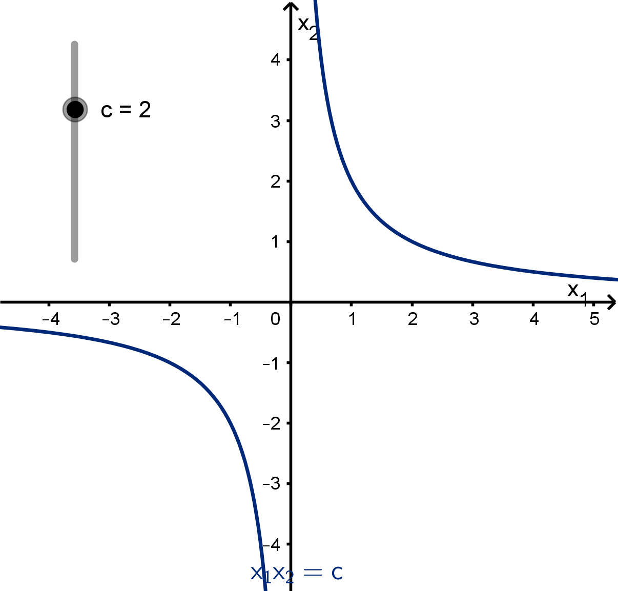
Figure 2.4: The level curves x

= c

Notice that x

= c is not always a curve. When c = 0, the level set is the x

- and x

-axes. At

the origin, this is two curves (lines) intersecting.

For a three-variable function, the level sets are called level surfaces because for most values of c,

they are 2-dimensional.

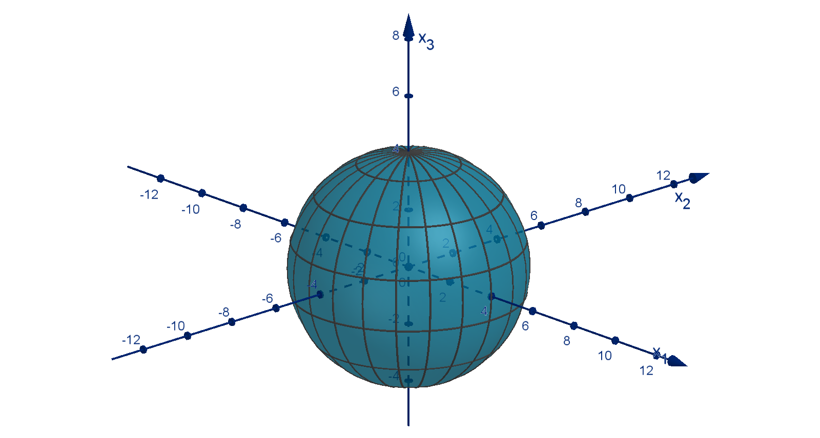
Figure 2.5: The level surfaces x

+ x

= c

Notice x

+ x

= 0 is not a surface, it is a point. x

+ x

= −5 is the empty set.

It can be diﬃcult to determine the shape and structure of a level set. A powerful mathematical

theorem can tell us when to expect good behavior.

Corollary 2.5 [Corollary to the Implicit Function Theorem]

Let g(x) be a continuously diﬀerentiable function at a. If a lies on the level set g(x) = c and ∇g(a) =



then the level set g(x) = c is a (n −1)-dimensional shape in some neighborhood of a. Speciﬁcally, it is

the graph of a diﬀerentiable function of n − 1 of the variables of R

This means that for smooth functions we can generally expect the level set to be a space of one

dimension lower than the domain, except at the occasional points where ∇g(x) =



0. We can see this

in our previous examples.

For g(x

, x

) = x

the nonempty level sets are curves, except for x

= 0. Even x

= 0

looks like a curve in any neighborhood that does not include (0, 0).

For g(x

, x

) = x

+ x

the nonempty level sets are surfaces (spheres), except for

+ x

= 0

We will give an argument for this corollary once we have seen the implicit function theorem in chapter

2.1.3

Finding the Maximizer and Minimizer Graphically

The level set g(x) = 0 is obviously important to a constrained optimization problem. We can also

use level sets to understand the shape of the objective function. Level sets have the advantage that

they live in R

, not R

n+1

, making them easier to draw than the graph y = f(x),

Consider the objective function f(x

, x

) = x

+ x

subject to x

− x

− 4 = 0.

What are the level curves of f (x

, x

How can we use a diagram of the level curves of f to argue that (1, −3) is not a local maximizer

or minimizer?

Where do the local maximizer(s) and local minimizer(s) of f on x

− x

− 4 = 0 appear to lie?

Are any of the local maximizers and minimizers also global maximizers or minimizer?

Solution

The level sets have the form x

= c these are circles centered at the origin, with higher values

the farther from the origin we go.

(1, −3) lies on the level set x

= 10. We can see from a sketch that the curve x

−x

−4 = 0

passes through this level set from higher values to lower values. Thus (1, −3) is not a local

maximizer or minimizer.

(0, −4) appears to be a local maximizer, because x

− x

− 4 = 0 meets the x

+ x

= 16 and

travels back to smaller-values in both directions. There also appear to be local minimizers in the

third and fourth quadrant where x

− x

− 4 = 0 touches a smallest level set and then travels

back to larger-valued level sets.

There is no global maximizer. As we travel upwards in x

−x

−4 = 0, we cross larger and larger

valued level sets. There is no upper bound to the values of f(x

, x

) that we can attain on the

constraint. On the other hand, the local minimizers are global minimizers. The only smaller-valued

level curves are inside that circle, and the constraint does not enter that region.

c = 1

c =?

c = 10

c = 16

c = 25

(1, −3)

global min global min

local max

Figure 2.6: Level curves of x

+ x

and the level curve x

− x

− 4 = 0

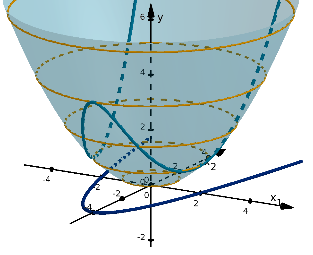
Figure 2.7: The graph of y = x

+ x

over the constraint x

− x

− 4 = 0

When the level set g(x) = 0 crosses a level set f(x) = c at a, this usually means that it intersects

2.1.3

Finding the Maximizer and Minimizer Graphically

both larger-valued and smaller-valued level sets on either side. If it does, then a cannot be a local

maximizer or minimizer of f on the constraint.

Main Idea

We expect to ﬁnd local maximizer and minimizers only where the level set g(x) = 0 is tangent to a level

set of f.

We can base our intuition on the following narrative: g(x) = 0 crosses higher and higher-valued level

sets of f as it approaches f(x) = c. When it reaches f (x) = c, rather than crossing it to even higher

values, it brushes against it (tangency) and backs away toward lower-valued level sets.

This does not describe every possible version of tangency. The curve x

− x

= 0 is tangent to

the level set x

= 0, but still crosses onto both sides. Furthermore level sets can behave unpredictably

when their gradient vector is



0. A rigorous argument for a maximizer using tangency generally needs to

appeal to the algebraic properties of f (x) and g(x) in some way.

2.1.4

The Lagrangian

Looking for tangency is a valuable method for approximating the maximizer, but we cannot expect it

to be precise enough to determine exact coordinates. For an exact position, we need a set of equations

to solve. These equations take the form of a necessary condition for a maximizer subject to an equality

constraint. We ﬁrst form a new function from both the objective function and the constraint.

Deﬁnition 2.6

Given an n-variable objective function f(x) and a constraint g(x) = 0, the Lagrangian is an (n + 1)-

variable function of the x

and λ (lambda). Its equation is

L(x, λ) = f(x) + λg(x)

Theorem 2.7

Let f(x) and g(x) be continuously diﬀerentiable functions. If a is a local maximizer or minimizer of

f(x) subject to the constraint g(x) = 0, then either

1 there is some number λ such that (a, λ) satisﬁes the ﬁrst-order condition of L or

2 ∇g(a) = 0.

We will call these the points that satisfy these conditions critical points or stationary points of

the constrained optimization problem. The value of λ is called a Lagrange multiplier.

Remark

Notice that this theorem is a necessary condition for a maximizer or minimizer, not a suﬃcient one.

2.1.5

Using the Lagrangian

We expect that the objective function f(x

, x

) = x

+ x

has a minimizer on the constraint

− x

− 4 = 0 somewhere in the fourth quadrant. Find it.

Solution

Letting g(x

, x

) = x

− x

− 4 we have the Lagrangian:

L(x

, x

, λ) = x

+ x

+ λ(x

− x

− 4)

∇g(x

, x

) = (2x

, −1). This is never



0, so any minimizer must satisfy the ﬁrst-order condition of L.

2.1.5

Using the Lagrangian

We set the partial derivatives equal to 0 and solve.

∂L

∂x

= 0

∂L

∂x

= 0

∂L

∂λ

= 0

+ 2x

λ = 0 2x

− λ = 0 x

− x

− 4 = 0

(1 + λ) = 0

if x

= 0 0

− x

− 4 = 0

= −4

if λ = −1 2x

+ 1 = 0

= −

− 4 = 0

= ±

The only possible local maximizers and minimizer are (0, −4),



, −



and



−

, −



. Since we

are looking for a minimizer in the fourth quadrant, it must be



, −



2.1.6

Proving the First-Order Condition of the Lagrangian

The partial derivatives of the Lagrangian are

∂L

∂x

(x) + λg

(x)

∂L

∂λ

=g(x)

Any solution (a, λ) to the ﬁrst-order condition on L satisﬁes

1 f

(a) = −λg

(a) for all i, so ∇f (a) = −λ∇g(a).

2 g(a) = 0, so a lies on the constraint.

The necessity of 2 is easy to explain. If a does not lie on the constraint, then it cannot be a

maximizer or minimizer subject to that constraint.

In order to understand 1 , we need to investigate the relationship between gradient vectors and

level sets. Like with multivariable unconstrained optimization, we use compositions over paths to study

maximizers on constraints. We need to alter our approach in three important ways.

100

We are only comparing f(a) to f(



b) for other



b in the level set g(x) = 0. Thus we only consider

paths x(t) that stay in the level set.

Unless the level set is linear, we cannot assume the paths x(t) are straight lines. They likely need

to curve to stay in the level set.

The tangent vectors x

′

(t) generally cannot point in all directions. Most directions of travel would

cause the path to leave the level set.

Now we examine the composition f(x(t)) where x(t) is a path in the level set g(x) = 0.

Figure 2.8: The composition f(x

(t), x

(t)) for a path (x

(t), x

(t)) in the level set g(x

, x

) = 0 and

its realization as the heights of y = f(x

, x

)

If a is a local maximizer or minimizer of f(x) among the points on g(x) = 0 then it must be a local

maximizer or minimizer of the composition f(x(t)) for all paths x(t) in the level set g(x) = 0. This

means the t-value corresponding to a (we will call it t

) must satisfy the ﬁrst-order condition of f(x(t)).

To compute the derivative of the composition, we apply the chain rule.

) = 0 (ﬁrst-order condition)

∇f(x(t

)) · x

′

) = 0 (chain rule)

∇f(a) · x

′

) = 0

In the unconstrained case, ∇f(a) · v = 0 for all v allowed us to conclude that ∇f(a) = 0. Our

conclusion cannot be so restrictive here. x(t) must be a path in the level set. We are thus only

considering vectors x

′

) that are tangent to the level set at a.

To make a conclusion about ∇f (a), we appeal to the geometric properties of the dot product. ∇f (a)

and x

′

) must be orthogonal for all paths in the level set that pass through a at t

. We introduce the

following vocabulary to describe this relationship between ∇f(a) and the level set.

101

2.1.6 Proving the First-Order Condition of the Lagrangian

Deﬁnition 2.8

A vector v is normal to a set at a, if v orthogonal to all tangent vectors of that set at a.

To avoid having to mention it as a separate case, we consider



0 to be orthogonal to every vector.

Lemma 2.9

If a is a local maximizer or local minimizer of a continuously diﬀerentiable function f(x) subject to

g(x) = 0, then ∇f(a) is normal to the level set g(x) = 0.

This gives us a good characterization of the gradient of the objective function at a local maximizer

or minimizer. We can now visually rule out a potential maximizer, if its gradient does not point in the

right direction. We now need to connect this to our computational tool. The Lagrangian compares ∇f

to ∇g. What can we say about ∇g?

Again, we consider a path x(t) in the level set g(x) = 0. This time we study the composition g(x(t)).

If you think carefully about what we have done, you will notice that this is a silly composition. We can

evaluate this composition at any value of t, and we will always get 0 (make sure you see why).

We can now apply the chain rule to g(x(t)), the zero function. This time the derivative is zero

because we are diﬀerentiating a constant function.

) = ∇g(x(t

)) · x

′

)

0 = ∇g(a) · x

′

)

We conclude that ∇g(x(t)) is orthogonal to x

′

(t) for all paths x(t) in the level set g(x) = 0.

Remark

This argument did not rely on a being any special point on the level set. Nor did it matter that the level

set had value 0. Any level set g(x) = c will have this relationship to the gradient, since the composition

will still be a constant function.

The result of this argument is the one of the most important geometric facts about gradient vectors.

We will use it over and over again.

102

Theorem 2.10

If g is a continuously diﬀerentiable function, and g(a) = c, then ∇g(a) normal to the level set g(x) = c.

In R

, this means that ∇g(a) points either 90

◦

degrees clockwise or 90

◦

counterclockwise from

x

′

Figure 2.9: Two possible ∇g(x(a)) orthogonal to x

′

)

In the case of a level surface, there are many paths through a. In order to be normal to the level

set, there are only two possible directions for ∇g(a).

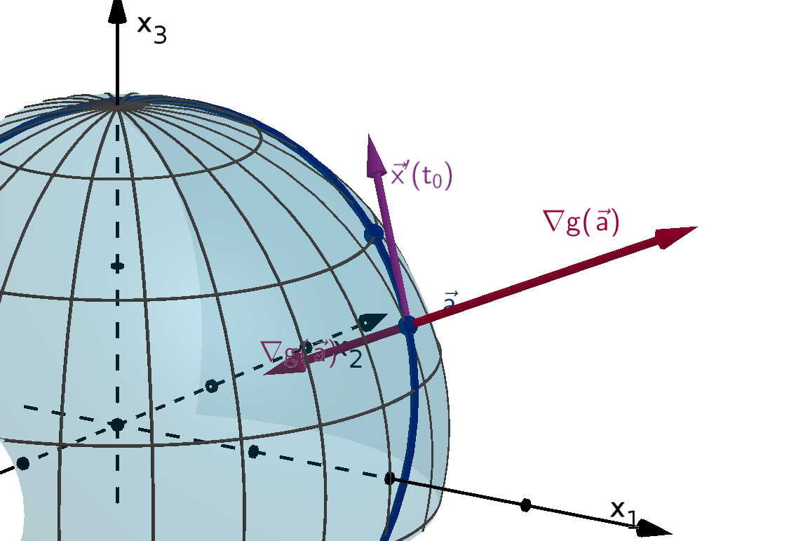
Figure 2.10: Two possible ∇g(a) orthogonal to all possible tangent vectors x

′

) in the level set

g(x) = 0.

We can use Corollary 2.5 to generalize this to an n-variable function. The level set is an (n − 1)

dimensional graph in n-space (as long as the gradient is nonzero). It has two normal directions, pointing

in opposite directions.

We can summarize what we have learned about the gradients of f and g as follows.

103

2.1.6 Proving the First-Order Condition of the Lagrangian

∇f(a) is normal to the level set g(x) = 0 at a local maximizer a.

∇g(x) is normal to the level set g(x) = 0 at all points on the level set.

If ∇g(a) =



0, then there are only two normal directions to the level set g(x) = 0, pointing in

opposite directions.

Vectors in the same or opposite directions are parallel. Algebraically, they are scalar multiples of each

other. We conclude that at any local maximizer or local minimizer, f(a) = −λ∇g(x) for some λ. This

is exactly what the ﬁrst-order condition of the Lagrangian requires.

Figure 2.11: Parallel vectors ∇f(x) and ∇g(x) at a minimizer of f(x) subject to g(x) = 0

This line of reasoning is complex. It is also important. We will revisit and generalize it later. Here

is a reminder of the steps of our argument.

a is a local maximizer

of f(x) on g(x) = 0

is a local maximizer of f(x(t))

on any path x(t) through a in g(x) = 0

f(x(t)) = 0 at t

∇f(a) · x

′

) = 0

∇f(a) is normal to g(x) = 0

∇g(x) is always

normal to g(x) = 0

There are only two

normal directions to g(x) = 0

∇f(a) and ∇g(a) are parallel

∇f(x) = −λ∇g(a) for some λ

(λ,a) satisﬁes the FOC

of the Lagrangian

FOC

chain rule

104

2.1.7

The Tangency Method

This argument also validates the tangency method of locating a maximizer. Theorem 2.10 applies

to f as well as to g. ∇f(a) is normal to the level set f(x) = c where c = f(a). At a local maximizer,

where ∇f (a) and ∇g(a) are parallel, it must follow that the level sets g(x) = 0 and f (x) = c have the

same normal directions. This implies that g(x) = 0 and f (x) = c are tangent to each other.

Corollary 2.11

Suppose both ∇f(a) and ∇g(a) exist and are not



0. If a is a maximizer of f(x) subject to g(x) = 0,

then the level sets of f and g that contain a are tangent to each other at a.

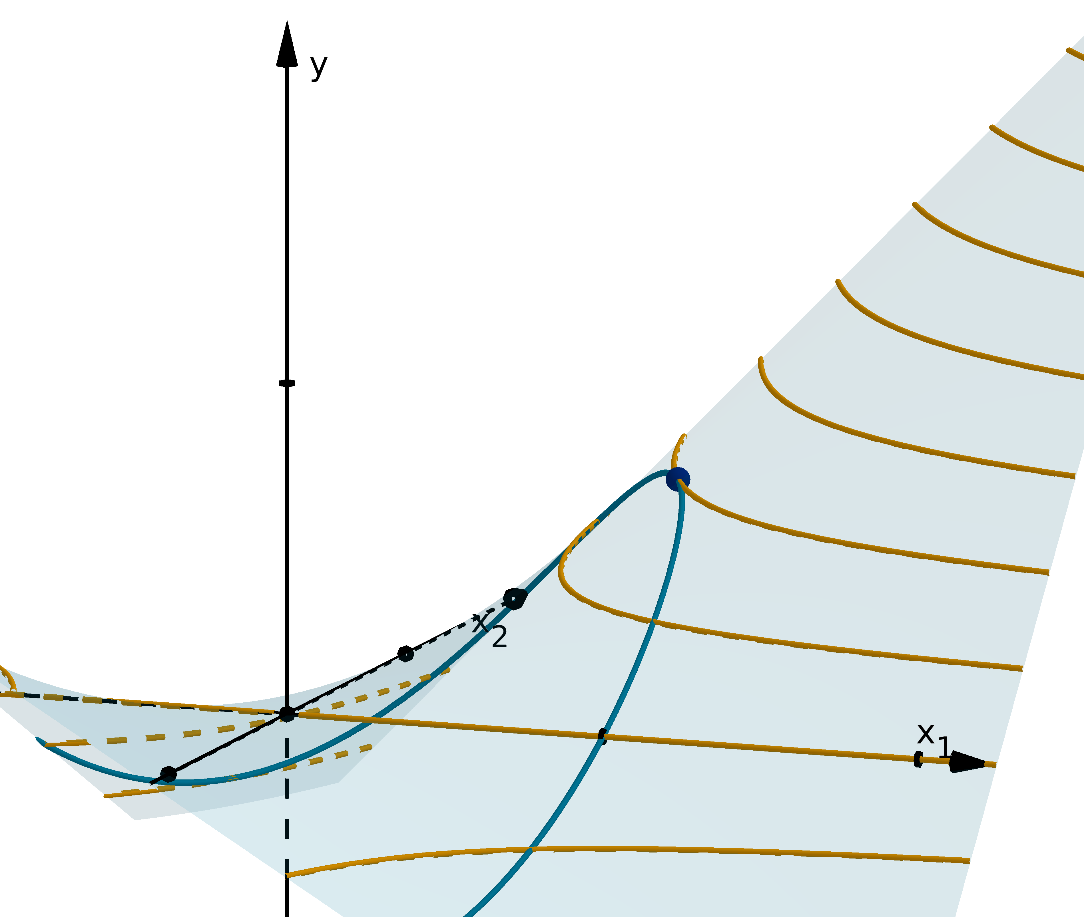
Figure 2.12: Parallel ∇f and ∇g and their tangent level curves at a local maximizer

2.1.8

Section Summary

The important deﬁnitions and results from this section were

The eﬀect of strengthening a constraint (Lemma 2.1)

The deﬁnition of a level set (Deﬁnition 2.4)

The Lagrangian (Deﬁnition 2.6)

The ﬁrst-order condition of the Lagrangian (Theorem 2.7)

The direction of the gradient (Theorem 2.10)

The tangency of level curves (Corollary 2.11)

105

2.2

Inequality Constraints

Goals:

1 Identify maximizers subject to inequality constraints.

2 Use the Lagrange multiplier to identify points that cannot be maximizers or minimizers.

3 Recognize several notations for complementary slackness.

2.2.1

Inequality Constraints and Upper Level Sets

Deﬁnition 2.12

An inequality constraint is a constraint of the form g(x) ≥ 0. With such a constraint we are solving

max

x∈D

f(x) subject to g(x) ≥ 0 or

max

x∈S

f(x) where S = {x ∈ D : g(x) ≥ 0}

Remark

Like with an equality constraint, just about any non-strict inequality can be rewritten in the form

g(x) ≥ 0. Even an expression g(x) ≤ k is equivalent to k − g(x) ≥ 0.

Here are two prototypical applications of inequality constraints in economics.

Example

If you have a budget to buy two types of goods, but you are not required to spend all of it, then your

constraint is

I − p

− p

≥ 0

106

Example

If x

denotes a physical quantity then it is often appropriate to assume

≥ 0.

Inequalities like these deﬁne the familiar shape of the budget set.

I/p

Figure 2.13: The region constrained by I − p

− p

≥ 0, x

≥ 0 and x

≥ 0

The set of points that satisﬁes an inequality constraint generally lies on one side of the level set

g(x) = 0. Graphically, it is the subset of the domain over which the graph y = g(x) is above the plane

y = 0. We therefore adopt the following terminology.

Deﬁnition 2.13

Given a multivariate function f(x) a upper level set of f is the set of points that, for some number

c, satisfy f(x) ≥ c. The points that satisfy f (x) ≤ c are a lower level set.

107

2.2.1

Inequality Constraints and Upper Level Sets

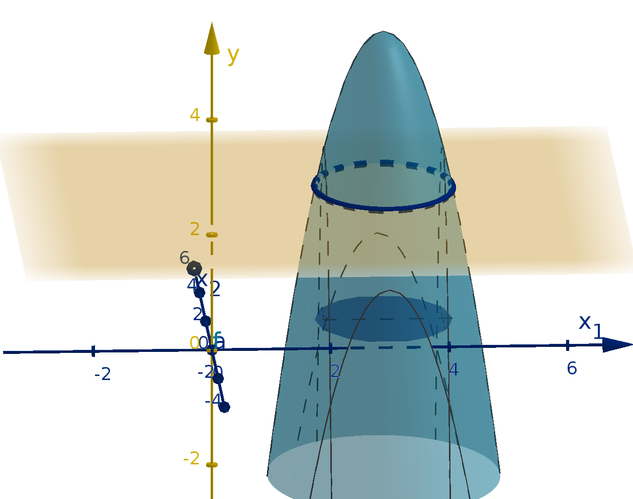
Figure 2.14: The upper level set where y = f (x) lies above y = c

We can use the chain rule to determine whether a path travels into an upper level set or lower level

set.

Lemma 2.14

Suppose a lies in the level set f(x) = c, ∇f(a) =



0, and x(t) is a path that passes through a at t

If x

′

) makes an acute angle with ∇f(a), then immediately after t

, x(t) travels into the upper

level set f(x) ≥ c.

If x

′

) makes an obtuse angle with ∇f(a), then immediately after t

, x(t) travels into the lower

level set f(x) ≤ c.

Figure 2.15: The gradient vector, the upper level set and the lower level set of f

108

The gradient vector makes an acute angle with itself, so we obtain the following characterization

immediately.

Corollary 2.15

Suppose f(a) = c. If ∇f(a) =



0, then ∇f(a) points into the upper level set f(x) ≥ c.

We can visualize the reasoning behind Lemma 2.14. Here is the case where the angle is acute.

x

′

) makes an acute

angle with ∇f(a)

∇f(a) · x

′

) > 0

In some nbhd of t

f(x(t)) > f(x(t

)) for t > t

In some nbhd of t

x(t) is in the upper level set

f(x) ≥ c for t > t

chain rule

Lem 1.2

2.2.2

Binding and Nonbinding Constraints

We already have the tools to impose necessary conditions on a maximizer subject to an inequality

constraint. Our strategy is to consider two cases and to apply the appropriate ﬁrst-order conditions to

each one.

Suppose a is a local maximizer of f(x) subject to g(x) ≥ 0.

1 If g(a) = 0 we say that the constraint is binding.

a

Figure 2.16: A maximizer a on g(x) = 0

109

2.2.2

Binding and Nonbinding Constraints

If a is a maximizer subject to g(x) ≥ 0, then it also maximizes f subject to g(x) = 0. It must

satisfy the FOC of the Lagrangian.

2 If g(a) > 0 then the constraint is non-binding.

x

′

(t)

a

Figure 2.17: A maximizer a in g(x) > 0 and some directions of travel through a

We can travel in all directions x

′

(t) through a without immediately leaving the upper level set.

To ensure ∇f(a) · x

′

(t) = 0, ∇f(a) must be the zero vector.

At an interior point, the boundary is not relevant to local measurements like the derivative. The

conditions of optimization are those of an unconstrained optimization, as if the constraint did not exist.

2.2.3

The Sign of λ at a Maximizer

If the inequality constraint g(x) = 0 binds at local maximizer a, then a will satisfy the ﬁrst-order

condition of the Lagrangian

L(x, λ) = f(x) + λg(x)

What can we say about the λ that goes with a?

Any path in the direction of ∇f(a) points toward higher values of f. If ∇f(a) points into the region

g(x) ≥ 0, then a cannot be a local maximizer subject to g(x) ≥ 0. This can be tested by the sign of λ.

∇g

∇f

a

Figure 2.18: A non-maximizing critical point a on g(x) = 0

110

The ﬁrst-order condition of the Lagrangian requires that ∇f (a) = −λ∇g(a). ∇g(a) points into the

upper level set g(x) ≥ 0. If λ is negative then ∇f (a) points into this set as well.

Lemma 2.16

Suppose that (a, λ) satisﬁes the ﬁrst-order condition of the Lagrangian of f subject to g(x) = 0. If a

is a local maximizer of f(x) subject to g(x) ≥ 0, then either

1 λ ≥ 0 or

2 ∇g(a) =



Understanding the intuition behind this result is probably more important than knowing a formal

proof. Still, here is a proof. Like the argument we have already given, it is a proof of the contrapositive.

Proof

If ∇g(a) =



0 then the lemma is satisﬁed. We will consider the case where ∇g(a) =



0 and λ < 0. We

will show that a is not a local maximizer.

Consider the line through a in the direction of ∇g(a). Its equation is x(t) = a + t∇g(a) and

x

′

(0) = ∇g(a). By Lemma 2.14, since ∇g(a) · x

′

(0) = ∇g(a) · ∇g(a) > 0, this line travels into the

upper level set g(x) ≥ 0 at t = 0.

What happens to values of f along this line? Consider the composition f(a+ t∇g(a)). Its derivative

at t = 0 is

(0) = ∇f(a) · ∇g(a)

= (−λ∇g(a)) · ∇g(a)

= −λ(∇g(a) · ∇g(a))

> 0

By Lemma 1.2, there is a neighborhood of 0 where for t > 0, f(x(t)) > f(x(0)) = f(a). We have seen

that these points lie in the upper level set, so a cannot be a maximizer of f(x) subject to g(x) ≥ 0.

Since a cannot be a maximizer when λ < 0, we conclude that if a is a maximizer, then λ ≥ 0.

Remark

Showing that a is not a maximizer required us to compare it to points in the upper level set g(x) ≥ 0.

This reasoning does not work when maximizing subject to an equality constraint. The line we used does

not lie in g(x) = 0. We can thus pout no restriction on λ when maximizing subject to g(x) = 0. λ can

be positive, negative, or zero at a maximizer.

111

2.2.4

Complementary Slackness

Whenever we have an inequality constraint, there are two cases to check: it can be binding or non-

binding. We could keep track of this manually, but there is an easier way to organize our search. We

can use the Lagrangian

L(x, λ) = f(x) + λg(x)

to test for both the binding and non-binding case.

g(x) ≥ 0 binding:

A maximizer a satisﬁes the ﬁrst-order

condition of the Lagrangian.

This automatically checks g(a) = 0.

We can check that λ ≥ 0.

g(x) ≥ 0 nonbinding:

We can set λ = 0

Now a maximizer a satisﬁes the ﬁrst-

order condition of L(x, λ) = f(x).

We can check that g(a) ≥ 0.

There is an interesting algebraic symmetry between the role of λ and g(a). The following deﬁnition

allows us to combine both these cases into one statement.

Deﬁnition 2.17

A point satisﬁes two non-strict inequalities with complementary slackness, if at least one of them

holds with equality.

We can cover both cases of an inequality constraint by demanding that g(x) ≥ 0 and λ ≥ 0 hold

with complementary slackness. Here are a few diﬀerent ways to denote complementary slackness.

Notations for Complementary Slackness

1 g(x) ≥ 0 and λ ≥ 0 hold with complementary slackness

2 g(x) ≥ 0, λ ≥ 0 and λg(x) = 0

3 λ ≥ 0 and g(x) ≥ 0, = 0 if λ > 0

112

2.2.5

Conditions for a Maximizer Subject to an Inequality Constraint

With complementary slackness in hand, we can write a necessary condition for a maximizer on an

inequality constraint. This theorem is written using notation 2 , but we could rewrite it with one of the

other notations.

Theorem 2.18

Let f(x) and g(x) be continuously diﬀerentiable functions. If a is a local maximizer of f(x) subject to

the constraint g(x) ≥ 0, then one of the following must be true

1 there is some number λ such that (a, λ) satisﬁes

∂L

∂x

(a, λ) = 0 for all i

g(a) ≥ 0, λ ≥ 0, and λg(a) = 0.

2 g(a) = 0 and ∇g(a) = 0.

2.2.6

Opimization Subject to an Inequality Constraint

Find the maximizer of f(x

, x

) = 10 − x

− x

subject to 3x

+ 4x

≥ 25.

Solution

First we write our constraint in the correct form. g(x

, x

) = 3x

+4x

−25 ≥ 0. Note that ∇g(x

, x

)

is never



0, so any critical point must satisfy our complementary slackness conditions. The Lagrangian is

L(x

, x

, λ) = 10 − x

+ x

+ λ(3x

+ 4x

− 25)

The conditions are

∂L

∂x

= 0

∂L

∂x

= 0

λ ≥ 0 3x

+ 4x

− 25 ≥ 0 λ(3x

+ 4x

− 25) = 0

113

2.2.6

Opimization Subject to an Inequality Constraint

First consider the λ = 0 case. The constraint is nonbinding. We solve the equations then check the

inequality.

∂L

∂x

= 0

∂L

∂x

= 0 λ = 0

−2x

+ 3λ = 0 −2x

+ 4λ = 0

−2x

= 0 −2x

= 0

= 0 x

= 0

check 3(0) + 4(0) − 25 ≥ 0

The only critical point we found failed the check. There is no maximizer where the constraint is

nonbinding. Now consider the g(x) = 0 case.

∂L

∂x

= 0

∂L

∂x

= 0 g(x) = 0

−2x

+ 3λ = 0 −2x

+ 4λ = 0 3x

+ 4x

− 25 = 0

λ x

= 2λ

λ + 8λ − 25 = 0

λ = 25

λ = 2

(2) x

= 2(2)

= 3 x

= 4

check λ ≥ 0

2 ≥ 0

The point (3, 4, 2) passes all of these conditions. We conclude that (3, 4) is the only possible maximizer.

Since this is not a suﬃcient condition, we cannot conclude (3, 4) is a maximizer. There may be no

maximizer at all.

Main Idea

To solve for the maximizer over an inequality constraint

1 Pick a case from complementary slackness

2 Set up and solve the system of equations

3 Check whether the solutions satisfy the inequalities

4 Repeat for the other case from complementary slackness

114

2.2.7

Section Summary

The important deﬁnitions and results from this section were

The notation of an inequality constraint (Deﬁnition 2.12)

The deﬁnition of an upper or lower level set (Deﬁnition 2.13)

The sign of λ at a maximizer subject to an inequality constraint (Lemma 2.16)

Complementary slackness (Deﬁnition 2.17)

Conditions for a maximizer on an inequality constraint (Theorem 2.18)

115

2.3

The Kuhn-Tucker Conditions

Goals:

1 Solve for maximizers on multiple constraints using the Kuhn-Tucker conditions

2 Recognize what each case of the Kuhn-Tucker conditions is checking

2.3.1

Multiple Equality Constraints

In economics, it is easy to imagine a ﬁrm is constrained by more than one equation:

A budget for capital and labor

Availability of labor or other inputs

A government regulation

You can’t purchase or produce a negative amount

What if we want to maximize an n-variable function f(x) subject to more than one equality con-

straint?

(x) = g

(x) = ··· = g

(x) = 0

The feasible set, is the intersection of the level sets g

(x) = 0. We have seen that a single level set

is usually one dimension less than the space it lies in. The intersection of m level sets will usually be an

(n − m)-dimensional shape.

Notation

The g

are diﬀerent functions, not partial derivatives of g. Whenever we have multiple g’s around, we

will need to write our partial derivatives using ∂ notation, for instance

∂

∂x

(x) not g

(x)

116

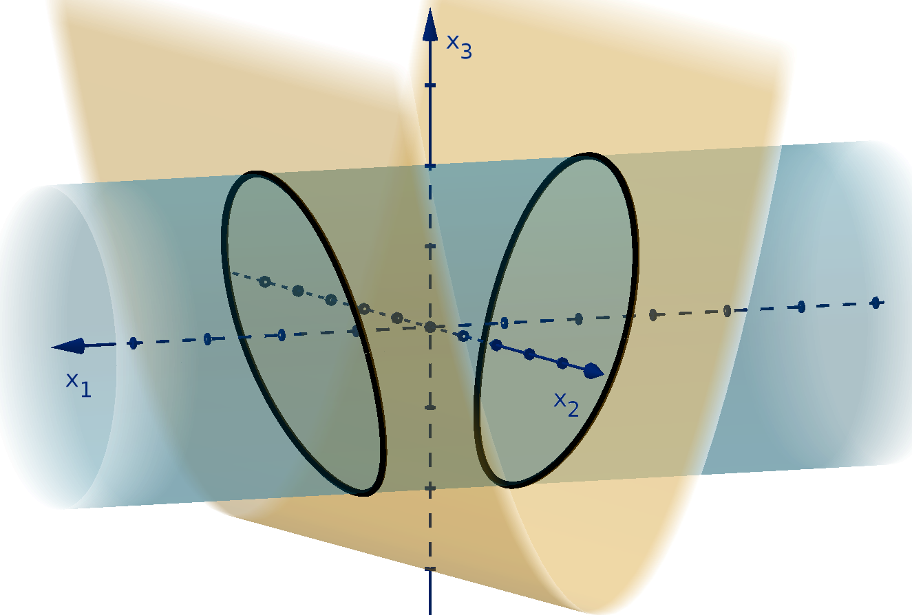
Figure 2.19: Two level sets intersecting at a pair of (one-dimensional) curves

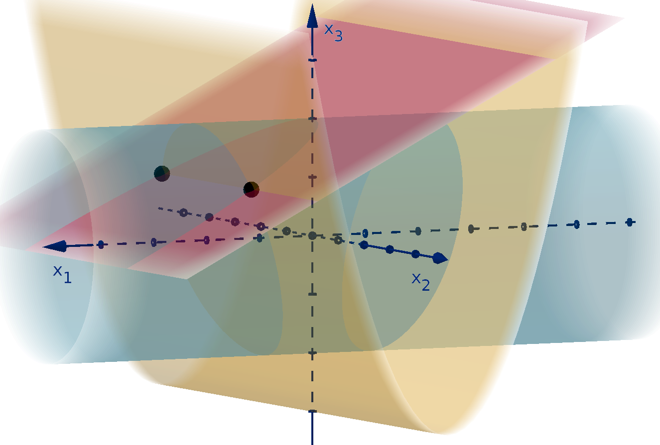
Figure 2.20: Three level sets intersecting at a pair of (zero-dimensional) points

Like with a single constraint, there are exceptions. Also like a single constraint, these exceptions

rely on the inadequacy of the gradient vector(s). The following deﬁnition come from linear algebra. A

corollary of the multivariable implicit function theorem characterizes the intersection of the level sets.

Deﬁnition 2.19

Vectors v

, v

, . . .v

are linearly dependent if there are constants k

, not all 0, such that

j=1

v



If no such k

exist then they are linearly independent

117

2.3.1 Multiple Equality Constraints

Equivalently, vectors are linearly dependent, if one of them is a linear combination of the others.

Corollary 2.20

Let g

(x), g

(x), . . . g

(x) be a continuously diﬀerentiable functions at a. If a lies on the level sets

(x) = c

and the ∇g

(a) are linearly independent, then the intersection of the level sets g

(x) = c

a (n −m)-dimensional shape in some neighborhood of a. Speciﬁcally, it is the graph of m diﬀerentiable

functions on R

n−m

Remark

Any set containing the zero vector is linearly dependent. Thus this corollary agrees with our criterion

for a single constraint. If the vector ∇g(a) =



0, then it is linearly dependent.

Two vectors are linearly dependent if they are parallel. With parallel gradients, the intersection of

m level sets can have fewer than (n − m) dimensions.

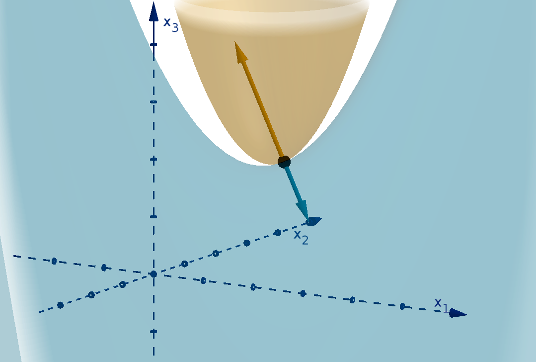
Figure 2.21: Two level sets with parallel gradients intersecting at a point

Parallel gradients can also occur when the level sets overlap, in this case the intersection can have

more than (n − m) dimensions.

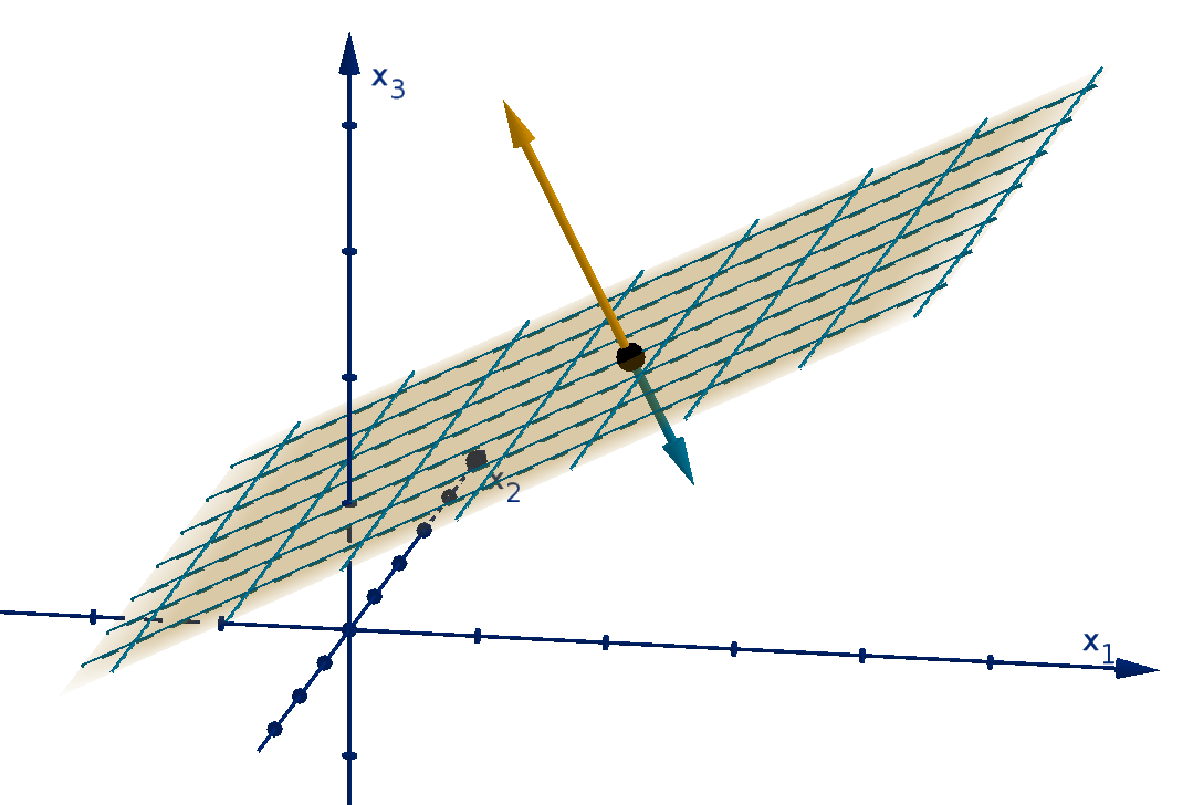
Figure 2.22: Two (overlapping) level sets whose intersection is a plane

118

Three vectors are linearly dependent if they are coplanar. Coplanar gradient vectors can also lead to

intersections of unexpected dimension.

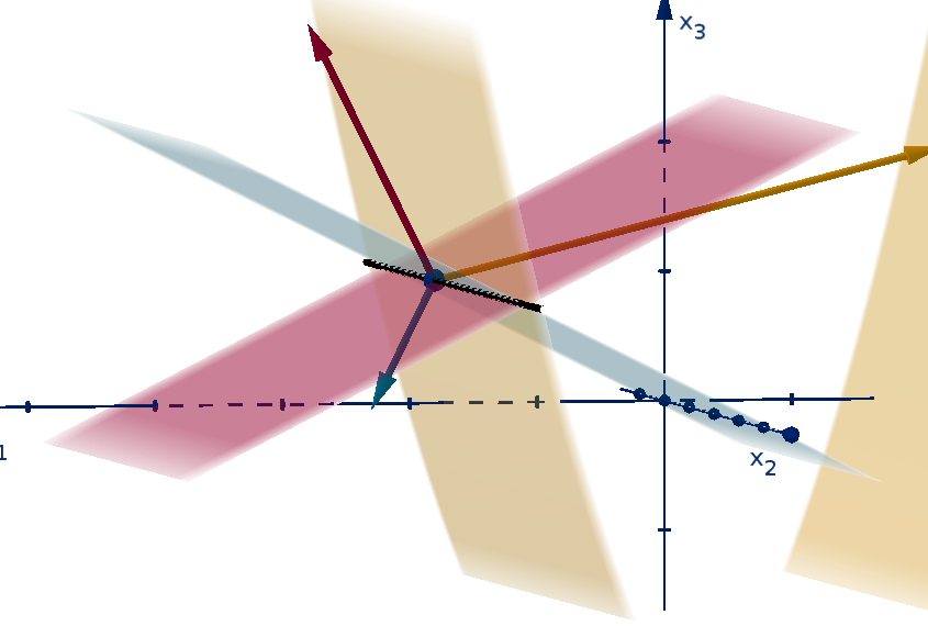
Figure 2.23: Three level sets with coplanar gradients intersecting on a line

Main Idea

Each additional equality constraint reduces the dimension of the feasible set by 1, unless its gradient

vector is a linear combination of the existing gradient vectors.

2.3.2

The Lagrangian for Multiple Equality Constraints

For multiple constraints, we write a Lagrangian that uses all of the constraints. We need a diﬀerent

variable λ for each one. The ﬁrst-order condition of this Lagrangian is a necessary condition for a local

maximizer or local minimizer.

Deﬁnition 2.21

Given the problem of maximizing an n-variable objective function f(x) subject to constraints g

(x) = 0

for 1 ≤ j ≤ m, the Lagrangian is a function of the n components of x and m variables



λ = (λ

, . . . , λ

L(x,



λ) = f(x) +

j=1

(x)

119

2.3.2 The Lagrangian for Multiple Equality Constraints

Theorem 2.22

If a is a local maximizer or local minimizer of f(x) subject to constraints g

(x) = 0, all continuously

diﬀerentiable at a, then either

1 (a,



λ) satisﬁes the ﬁrst-order condition of L for some



λ or

2 The ∇g

(a) are linearly dependent

Notation

When developing the theory, we write our constraint functions and our Lagrange multipliers using a

common letter and an index variable

(x), g

(x), . . . λ

, λ

, . . .

This makes it easier to generalize to any number of constraints, because can use Σ notation in the

Lagrangian. For a small number of constraints, using an index is inconvenient. Economists often use

diﬀerent letters for each constraint and multiplier.

g(x), h(x), . . . λ, µ, . . .

2.3.3

A Multi-Constraint Optimization

Find the maximizer of f(x

, x

) = 3x

on the constraints x

−50 = 0 and x

= 0.

Solution

The Lagrangian is

L(x

, x

, λ

) = 3x

+ λ

+ x

− 50) + λ

+ x

)

The ﬁrst-order condition is

120

∂L

∂x

= 0

∂L

∂x

= 0

∂L

∂x

= 0

∂L

∂λ

= 0

∂L

∂λ

= 0

2λ

+ λ

= 0 3 + λ

= 0 2λ

+ λ

= 0 x

+ x

− 50 = 0 x

+ x

= 0

= −3

2λ

= x

+ x

− 50 = 0

= ±5

±5 = x

±5 + x

± 5 = 0

= ∓10

We conclude that (±5, ∓10, ±5). The value f(x

, x

) = 3x

is larger when x

= 10. We conclude

that no point besides (−5, 10, 5) can be the maximizer of f on these constraints. Because this is not a

suﬃcient condition, we cannot be sure that this is the maximizer. It may be that no maximizer exists

at all.

We can visualize the maximizer of f(x

, x

) = 3x

by looking for the point in the level sets that

is farthest in the x

direction. It appears that such a point exists at (−5, 10, −5).

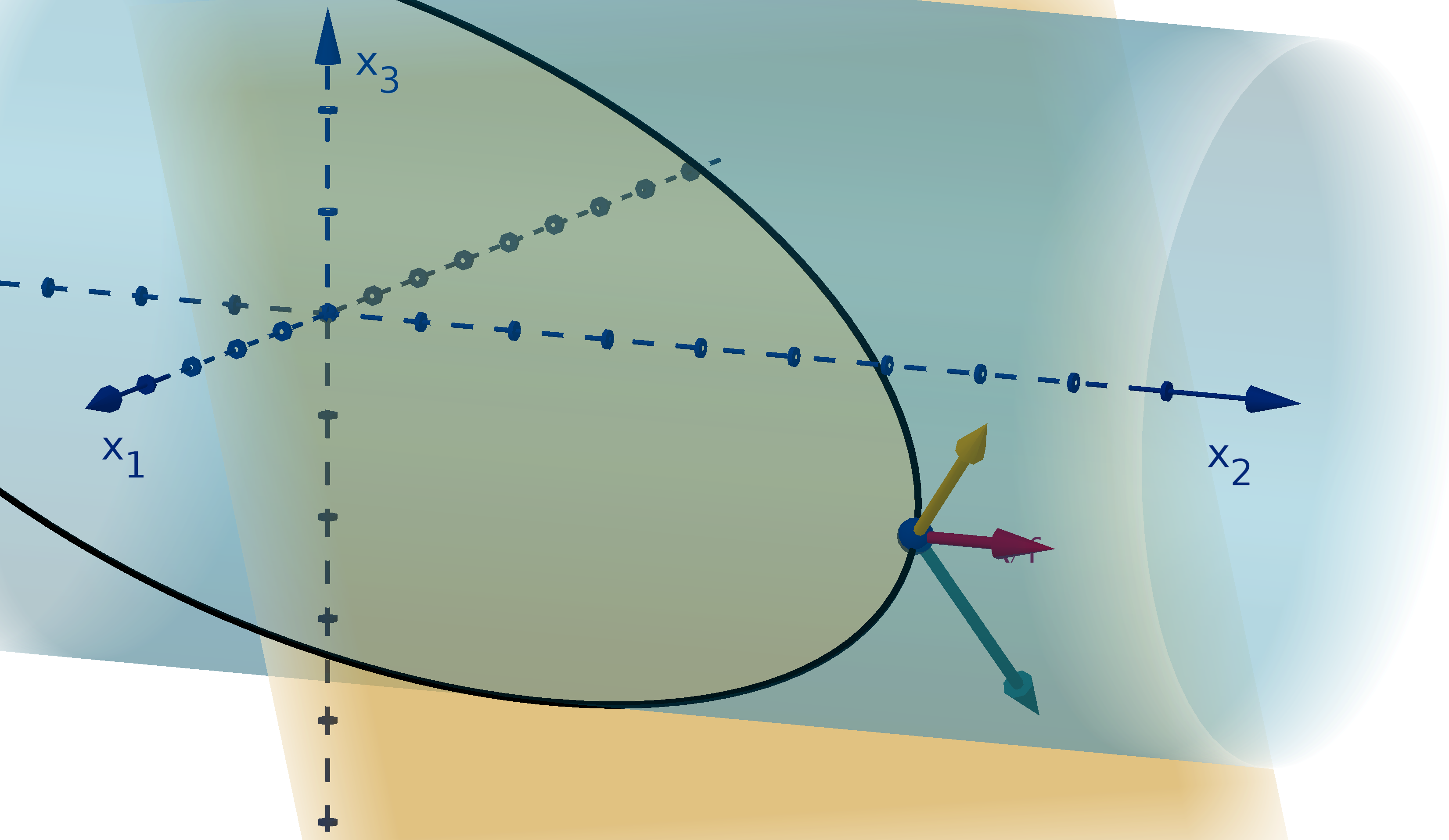
Figure 2.24: The gradients of x

+ x

− 50, x

+ x

= 0, and f(x) = 3x

at the maximizer

121

2.3.4

The Reasoning for the Multi-Constraint Lagrangian

The partial derivatives of the Lagrangian are

∂f

∂x

(x) +

j=1

∂g

∂x

(x)

Any solution (a,



λ) to the ﬁrst-order condition on L satisﬁes

(a) = −

j=1

∂g

∂x

(a) for all i, so ∇f (a) = −

∇g

(a).

(a) = 0 for all j so a lies on all the constraints.

We can examine the relationship between the gradients using the same procedure we used for a

single constraint. We take a path x(t) through a at t

. We assume that x(t) lies in the feasible set.

This means it lies in all of the level sets g

(x) = 0.

If a is a local maximizer or minimizer of f(x) on the feasible set then it must be a local maximizer

or minimizer of the composition f(x(t)) for all paths x(t) in the feasible set. This means the t-value

corresponding to a (we will call it t

) must satisfy the ﬁrst-order condition of f(x(t)). The derivative

calculation should be familiar:

0 =

)

0 = ∇f(x(t

)) · x

′

)

0 = ∇f(a) · x

′

)

Thus ∇f(a) is normal to the feasible set.

When we had a single constraint, we argued that there were two opposite normal directions to the

feasible set, and ∇g(a) pointed in one of them. This relied on the fact that our feasible set was a level

set and had dimension (n −1). If we assume that the ∇g

(a) are linearly independent, then the feasible

set has dimension (n − m) at a.

There is an entire m-dimensional space of vectors normal to the feasible set at a. If a is a maximizer,

∇f(a) must be a vector in this space.

122

Figure 2.25: The gradient vector of the objective function and the normal plane of the feasible set at a

local maximizer of the composition: f(x(t))

The feasible set lies in each level set g

(x) = 0. The gradient of each g

is normal its level set. We

can put together what we know about the gradients and the shape of the feasible set.

f(a) is normal to the feasible set at a local maximizer a.

Each ∇g

(x) is normal to the feasible set at all points in the level set.

If the ∇g

(a) are linearly independent, then the normal space is m-dimensional.

m independent vectors in a m-dimensional space must span the space. We conclude that ∇f(a) is a

linear combination of the ∇g

(a). This is what the ﬁrst-order condition of the Lagrangian requires.

Example

If a is a maximizer of a three-variable function subject to two equality constraints, then ∇f (a) must lie

in the normal plane, which is spanned by ∇g

(a) and ∇g

(a).

123

2.3.4 The Reasoning for the Multi-Constraint Lagrangian

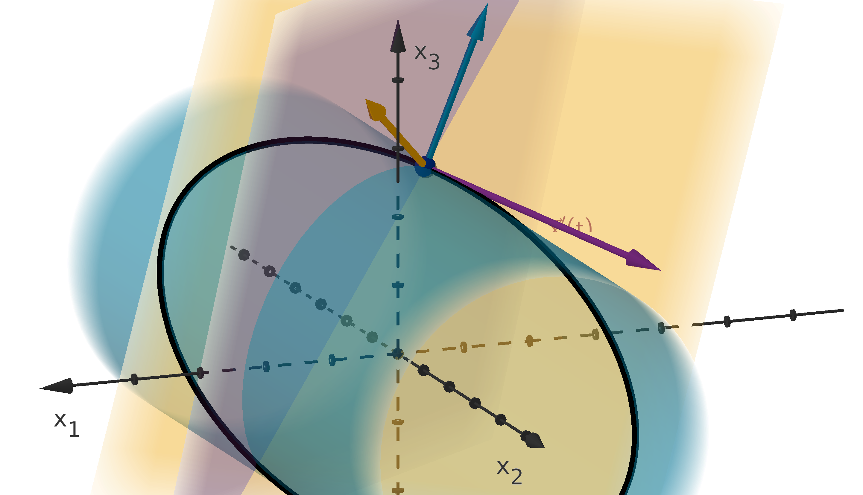
Figure 2.26: Two gradients spanning the normal plane of the feasible set

2.3.5

An Optimization with Dependent Gradients

When the gradients of the g

(x) are linearly dependent, the feasible set may not have the expected

dimension of (n − m). Even if it does, the gradient vectors need not span the normal space. In this

case, calculus arguments cannot rule out a point from being a maximizer. Here is an example where

insisting upon the ﬁrst-order condition of the Lagrangian would incorrectly rule out a maximizer.

Consider the smooth function f(x

, x

) = x

+ x

and the constraints x

+ 2 = 0 and x

− (x

−

+ 2 = 0. If we attempt to apply the ﬁrst-order condition we obtain the following.

The constraints intersect only at (3, −2).

At (3, −2) the gradients are

∇g

(3, −2) = (0, 1) ∇g

(3, −2) = (0, 1) ∇f(3, −2) = (6, −4).

∇f cannot be written as a linear combination of ∇g

and ∇g

Even though it doesn’t satisfy the ﬁrst-order condition, (3, −2) must be the maximizer (and mini-

mizer), since it is the only point that satisﬁes both constraints.

124

Figure 2.27: (3, 2) is a maximizer, but ∇f cannot be written λ

∇g

+ λ

∇g

If we count dimensions, the feasible set is a 0-dimensional subspace of R

. Its normal space is

2 − 0 = 2-dimensional, which suggests that ∇f(3, −2) can be any vector in R

. This sounds bizarre

but actually makes sense. (3, −2) is the entire feasible set. It must be a maximizer, no matter what

∇f(3, −2) is. The exception for dependent gradients in Theorem 2.22 exists to avoid ruling out a

maximizer in a situation like this.

2.3.6

The Kuhn-Tucker Conditions

The Kuhn-Tucker conditions are a robust set of necessary conditions for constrained optimizations

with inequality constraints, potentially in addition to some number of equality constraints. They combine

all of the ideas we have developed in this chapter. We will use the same Lagrangian that we would for

equality constraints.

A Lagrangian For Multiple Equality and Inequality Constraints

Given an objective function f(x) and constraints of the forms g

(x) ≥ 0 or g

(x) = 0 the Lagrangian

L(x,



λ) = f(x) +

j=1

(x).

Like with a single inequality constraint, complementary slackness will remove the λ

(x) when g

(x)

does not bind.

125

2.3.6 The Kuhn-Tucker Conditions

Theorem 2.23 [The Kuhn-Tucker Conditions]

Given the objective function f (x) and constraints of the forms g

(x) ≥ 0 or g

(x) = 0, then at any

local maximizer a one of the following must be true

1 There is some vector



λ such that (a,



λ) satisﬁes the Kuhn-Tucker conditions:

For each variable x

(a,



λ) = 0

For each equality constraint function g

(a) = 0

For each inequality constraint function g

(a) ≥ 0 and λ

≥ 0 and λ

(a) = 0

2 The binding ∇g

(a) are linearly dependent

2.3.7

Solving the Kuhn-Tucker Conditions

According to Kuhn-Tucker, what points (x

, x

) could be maximizers of f(x

, x

) = x

given the

constraints

12 − x

− 4x

≥ 0 9 − x

− x

≥ 0

Solution

The Lagrangian is L(x

, x

, λ

) = x

+ λ

(12 −x

−4x

) + λ

(9 −x

−x

). The Kuhn-Tucker

conditions are

∂L

∂x

= x

− λ

= 0

∂L

∂x

= 2x

− 4λ

− λ

= 0

12 − x

− 4x

≥ 0 9 − x

− x

≥ 0

≥ 0 λ

≥ 0

(12 − x

− 4x

) = 0 λ

(9 − x

− x

) = 0

The ﬁnal equations carry our complementary slackness conditions. There are two ways to choose which

factor is 0 for each, giving us 2 × 2 = 4 cases to check.

126

1 λ

= 0, λ

= 0

− λ

= 0 2x

− 4λ

− λ

= 0

= 0 2x

= 0

check 12 − x

− 4x

≥ 0 6 − x

− x

≥ 0

12 − x

≥ 0 6 − x

≥ 0

≤ 12 x

≤ 9

So (k, 0, 0, 0) satisﬁes the Kuhn-Tucker conditions for k ≤ 9.

2 λ

= 0, 9 − x

− x

= 0

− λ

= 0 2x

− 4λ

− λ

= 0 9 − x

− x

= 0

− λ

= 0 2x

− λ

= 0

= 2x

− 2x

= 0

− 2x

) = 0

= 0 covered in case 1

or x

= 2x

9 − x

− 2x

= 0

= 3

= 6

− λ

= 0

= 36

check 12 − x

− 4x

≥ 0 λ

≥ 0

12 − 3 − 4(6) ≥ 0 36 ≥ 0

−15 ≥ 0

(3, 6, 0, 36) does not satisfy the inequalities.

127

2.3.7

Solving the Kuhn-Tucker Conditions

3 12 − x

− 4x

= 0, λ

= 0

− λ

= 0 2x

− 4λ

− λ

= 0 12 − x

− 4x

= 0

− λ

= 0 2x

− 4λ

= 0

= 4λ

= 2x

− 2x

= 0

(2x

− x

) = 0

= 0 covered in case 1

or 2x

= x

12 − 2x

− 4x

= 0

= 2

= 4

− λ

= 0

= 4

check 9 − x

− x

≥ 0 λ

≥ 0

9 − 4 − 2 ≥ 0 4 ≥ 0

(4, 2, 4, 0) satisﬁes the Kuhn-Tucker conditions

4 12 − x

− 4x

= 0, 9 − x

− x

= 0

− λ

= 0 2x

− 4λ

− λ

= 0 12 − x

− 4x

= 0 9 − x

− x

= 0

12 − x

− 4x

= 0

−(9 − x

− x

) = −0

3 − 3x

= 0

= 1

9 − x

− 1 = 0

= 8

1 − λ

− λ

= 0 16 − 4λ

− λ

= 0

−(16 − 4λ

− λ

) = −0

−15 + 3λ

= 0

= 5

16 − 4(5) − λ

= 0

= −4

check λ

≥ 0 λ

≥ 0

5 ≥ 0 −4 ≥ 0

(8, 1, 5, −4) does not satisfy the Kuhn-Tucker conditions.

The Kuhn-Tucker conditions are necessary. No point except (4, 2) or (k, 0) for k ≤ 9 can be a maximizer.

128

By evaluating we see

f(4, 2) = 16 f(k, 0) = 0

So only (4, 2) could be a maximizer. We cannot conclude that it is a maximizer, until we learn a relevant

suﬃcient condition.

Strategy

In general our method for solving the Kuhn Tucker conditions is

Pick an equality from a factor of each complementary slackness condition.

Solve the resulting system of equations.

Discard any solutions that violate the remaining inequalities.

Repeat for a diﬀerent choice of equalities.

With m inequality constraints, we will need to repeat for all 2

combinations of equalities.

2.3.8

Visualizing the Kuhn-Tucker Conditions

Each choice of equalities mutates the Kuhn-Tucker conditions into the necessary conditions from

Theorem 2.22, where the binding g

(x) ≥ 0 are treated as equality constraints. The following diagram

shows how each choice corresponds to a diﬀerent piece of the feasible set, where diﬀerent constraints

bind.

∇g

(x) ≥ 0 and λ

= 0

(x) = 0 and λ

≥ 0

L(x,



λ) = f(x) + λ

(x)

∇f(x) = −λ

∇g

(x)

(x) ≥ 0 and λ

= 0

(x) ≥ 0 and λ

= 0

L(x,



λ) = f(x)

∇f(x) =



(x) = 0 and λ

≥ 0

(x) = 0 and λ

≥ 0

L(x,



λ) = f(x) + λ

(x) + λ

(x)

∇f(x) = −λ

∇g

(x) −λ

∇g

(x)

(x) = 0 and λ

≥ 0

(x) ≥ 0 and λ

= 0

L(x,



λ) = f(x) + λ

(x)

∇f(x) = −λ

∇g

(x)

Figure 2.28: The four regions covered by two pairs of inequalities with complementary slackness

129

2.3.8 Visualizing the Kuhn-Tucker Conditions

In the case of multiple binding inequality constraints, the condition that λ

≥ 0 forces ∇f(a) to lie

in the cone made by −∇g

(x).

∇g

−∇g

∇f

Figure 2.29: The cone where ∇f must lie if both constraints bind at a maximizer

2.3.9

Proving the Necessity of the Kuhn-Tucker Conditions

To justify the necessity of the Kuhn-Tucker conditions, we can list each condition and describe why

it must apply.

1 A given a will satisfy some binding equations g

(x) = 0.

2 For the constraints that do not bind, setting λ

= 0 turns L(x,



λ) into the Lagrangian for f with

only the binding equality constraints. If a is a local maximizer, it must satisfy Theorem 2.22,

speciﬁcally,

∂L

∂x

(a) = 0.

3 For each inequality constraint, a maximizer must satisfy g

(a) ≥ 0 to be feasible.

4 Finally, if every path from a into the feasible region decreases f , then all λ

≥ 0.

We have not given a convincing argument for the last statement yet. A formal proof is just below,

but it may be more illuminating to convince yourself graphically. Try drawing a few ∇f that lie outside

the cone between −∇g

and −∇g

in the previous ﬁgure. For each one, you should be able to identify

a vector x

′

(t) that points into the feasible region but makes an acute angle with ∇f.

Here is a formal proof that λ

≥ 0 at a maximizer.

Proof

Pick any inequality constraint g

(x) ≥ 0. If g

(x) ≥ 0 is not binding at a, then λ

= 0 and we are

done.

130

We will therefore consider the case where g

(a) ≥ 0 is binding and show λ ≥ 0. Let S be the inter-

section of all the binding constraints except g

(x) = 0. Since the gradients of the binding constraints

a linearly independent, we can conclude:

The gradients of the binding constraints other than ∇g

(a) span the normal space of S at a

∇g

(a) is not a linear combination of these gradients, so it does not lie in the normal space of S

at a

There must be a path x(t) in S through a such that x

′

) is not orthogonal to ∇g

(a). We can pick

such a path so that ∇g

(a) · x

′

) > 0. If the ﬁrst path we try produces a negative dot product, just

traverse x(t) backwards instead. First we show that, in some neighborhood of t

, x(t) lies in the feasible

region for all t > t

. We check that it satisﬁes each constraint.

a lies in the interior of each upper level set g

(x) ≥ 0 for each nonbinding g

. x(t) will travel for

some distance before leaving the upper level set.

Since x(t) was chosen to lie in S it lies in the level set g

(x) = 0 for all binding g

except g

Since ∇g

(a) · x

′

) > 0, x(t) must travel into the upper level set g

(x) ≥ 0.

Thus in some neighborhood of t

, x(t) lies in the feasible set for t > t

. Since a is a local maximizer,

f(x(t

)) ≥ f(x(t)) for t > t

in this neighborhood. Thus

) ≤ 0. We use the chain rule to examine

this inequality.

) ≤ 0

∇f(a) · x

′

) ≤ 0

−

j=1

∇g

(a) · x

′

) ≤ 0

We pause to examine the terms of this summation. Most are 0. Here is the reasoning.

For nonbinding g

(x), λ

= 0.

For binding g

(x) except j = m, we have ∇g

(a) ·x

′

) = 0, since ∇g

(a) is a normal vector of

S and x(t) lies in S.

Finally, ∇g

(a) · x

′

) > 0 by our choice of x(t).

We apply these to our inequality.

−

j=1

∇g

(a) · x

′

) ≤ 0

−λ

∇g

(a) · x

′

) ≤ 0

≥ 0

131

2.3.10

Kuhn-Tucker with Non-Negativity Constraints

If we demand that x

≥ 0 for each i, then we have added n new constraints to our Langrangian.

We will use µ

for the Lagrange multipliers of the x

L(x,



λ, µ) = f(x) +

j=1

(x) +

i=1

This is unwieldy. If we are clever, we can do better.

For 1 ≤ k ≤ n, the inequality conditions for µ

are

∂L

∂µ

= x

≥ 0 and µ

≥ 0

If the constraint x

≥ 0 is not binding, then µ

= 0. The µ

term is 0 in L and its partial

derivatives. We can remove it, but we will still need to verify that x

≥ 0 is satisﬁed.

If the constraint is binding, then we can still remove the µ

term from L.

The term goes to 0 anyway in L

for i = k.

In L

, there is a single +µ

term. L

is supposed to be 0, whereas µ

≥ 0. We can

replicate this eﬀect by removing µ

from L, but requiring that the remaining terms of L

have a sum less than or equal to 0.

For each k, we can remove the variable µ

and the µ

term from our Lagrangian in exchange for

some new conditions.

132

Corollary 2.24 [The Kuhn-Tucker Conditions with Non-Negativity]

Given the objective function f (x) and constraints of the forms g

(x) ≥ 0 or g

(x) = 0, along with

≥ 0 for each i, then at any local maximizer a one of the following must be true.

1 There is some vector



λ such that (a,



λ) satisﬁes the Kuhn-Tucker Conditions with Non-

Negativity Constraints:

For each i,

≥ 0 and

∂L

∂x

(a,



λ) ≤ 0 and a

∂L

∂x

(a,



λ) = 0

For each equality constraint function g

(a) = 0

For each inequality constraint function g

(a) ≥ 0 and λ

≥ 0 and λ

(a) = 0

2 The binding constraints (including any x

= 0) have linearly dependent gradients at a.

2.3.11

Section Summary

The most important deﬁnitions and results from this section were

The shape of an intersection of level sets (Corollary 2.20)

The Lagrangian for multiple constraints (Deﬁnition 2.21)

First-order condition for multiple equality constraints (Theorem 2.22)

The Kuhn-Tucker conditions (Theorem 2.23)

The Kuhn-Tucker conditions with non-negativity (Corollary 2.24)

133

2.3.11

Section Summary

134

Chapter 3

Comparative Statics

3.1

The Implicit Function Theorem

Goals:

1 Identify when one variable of an implicit equation can be written as a function of the other(s)

2 Compute the derivative of one variable with respect to another

3 Determine how the optimal choice responds to changes in an exogenous parameter

3.1.1

Comparative Statics

Comparative statics study situations with one or more choice variables x

and one or more exoge-

nous parameters α

Example

A consumer maximizing her utility has the choice variable

q: the quantity of a product they buy

and the exogenous parameter

p: the price of that product

136

Example

From the point of view of a producer, the choice variables might be

q: the quantity of a product they produce

p: the price they sell for

the exogenous parameters may include

w, r: the price of labor or capital

t, s: a tax or subsidy imposed by the government

some aspect of the demand function

Remark

The choice variables are the variables whose value is chosen by the agent who wants to maximize the

function.

In economics, we assume that choosers are rational and well-informed. We assume they will learn the

value of the parameters. After that, they will pick the value of the choice variables that maximizes their

objective function. Comparative statics ask how the outcome changes as the value of the parameter

changes. We will present the tools to compute two types of comparative statics

1 How does the optimal value of a choice variable change as a parameter changes?

2 How does the value of the objective function change as a parameter changes?

Notation

Given an objective function f(x, α), with choice variable x and parameter α, we expect that diﬀerent

values of α will lead the chooser to pick diﬀerent values of x. The chooser’s optimal choice is a function

of α that we write x

∗

(α).

The ﬁrst-order condition tells us that for each α, x

∗

(α) must satisfy the ﬁrst-order condition:

∗

(α), α) = 0

Without an expression for x

∗

(α), trying to understand its rate of change raises a sequence of questions.

1 What is

∗

(α)

dα

137

3.1.1

Comparative Statics

2 How do we know that x

∗

(α) is diﬀerentiable?

3 How do we know that x

∗

(α) is even a function?

Given a speciﬁc f, we can solve the ﬁrst-order condition algebraically. If we can tell which solution

is the maximizer (assuming one exists), then we can write an expression for x

∗

as a function of α and

answer all these questions. In the case of a general or abstract f, this may not be possible. Fortunately,

mathematics has the vocabulary to describe these questions in abstract. It also has a powerful tool to

answer them.

3.1.2

Explicit Functions and Implicit Equations

Deﬁnition 3.1

An explicit function equates a function or dependent variable to an expression entirely in terms of the

independent variables.

Example

The following equations describe explicit functions.

f(x) = x

−

√

x + 7

y = sin(x

)

z = 3xy + x

− 2

g(x

, x

) = e

cos(x

)

Since each input has at most one output, graphs of explicit functions pass the vertical line test. We

also have a variety of tools for diﬀerentiating explicit functions (though not all are diﬀerentiable).

We do not have the luxury of always working with explicit functions. We use the following vocabulary

when we wish to draw a contrast with explicit functions.

Deﬁnition 3.2

An implicit equation in two or more variables does not necessarily have any dependent variable which

is equated to an expression in the others.

Sometimes we can solve an implicit equation to obtain an explicit function, but other times we

cannot.

138

Example

2x + 3y = 12 =⇒ y = 4 −

+ x

= 25 =⇒ x

= ±

25 − x

− x

(multiple outputs for each input, not a function)

13 − 3y

+ xy

= y

=⇒ x =

− 13 + 3y

(can solve for x but not for y)

+ y

= 6xy =⇒ y = ??? (requires the cubic formula, not a function)

The solutions to any implicit equation form a level set of some function. We obtain the function by

rewriting the equation in a form like:

F (x, y) = c or F (x) = c

3.1.3

An Implicit Equation

Consider the implicit equation x

+ y

= 6xy

Write the equation in the form F (x, y) = c.

Does this equation have a graph?

Can we solve it to obtain an explicit function?

Solution

We can write x

+ y

− 6xy = 0

Yes. The graph is the set of points (x, y) that satisfy the equation. Every equation has a graph,

though some graphs are the empty set.

139

3.1.3

An Implicit Equation

We could look up the cubic formula and solve this. The cubic formula, like the quadratic formula,

returns multiple values for the variable. The result is not a function. We can see this in the graph,

which fails the vertical line test.

Figure 3.1: The graph of x

+ y

− 6xy = 0

Sometimes we cannot write y as an explicit function of x in a way that describes the whole graph.

If we are only interested in rates of change, we can restrict our attention to a small neighborhood of the

graph. At most points, this neighborhood does look like the graph of some function y = f (x).

Figure 3.2: A neighborhood in which the graph x

+ y

− 6xy = 0 is the graph of an explicit function

This is not always possible. Consider the part of x

+ y

−6xy = 0 near (0, 0). In any neighborhood

we choose, there are three branches of the graph that extend to the right. No matter how small a

neighborhood we choose around (0, 0), the graph will fail the vertical line test and cannot be written as

y = f(x).

140

3.1.4

The Implicit Function Theorem

The implicit function theorem tells us when a point on the graph of an implicit equation has a

neighborhood that is identical to the graph of an explicit function. The basic version takes an implicit

equation in two variables and writes a function that expresses one (the dependent variable) in terms of

the other (the independent variable).

Theorem 3.3 [The Implicit Function Theorem]

Suppose F (x, y) is a continuously diﬀerentiable function and (a, b) is a point on F (x, y) = c. If

(a, b) = 0, then there exists a diﬀerentiable function f (x) such that y = f(x) and F (x, y) = c

describe the same graph in some neighborhood of (a, b).

The theorem does not tell us what the function f(x) is, only that it exists. Even so, we can express

its derivatives in terms of F .

Corollary 3.4

The derivative of f with respect to x at a is given by

′

(a) = −

(a, b)

The derivation of this formula is famous and not too diﬃcult. To compute the derivative of f, we

parameterize a path in the graph y = f(x). Unlike our previous parametrizations, we will use x as the

parameter. Diﬀerentiating x with respect to x is most palatable with Leibniz notation.

x = x

= 1

y = f(x)

= f

′

(x)

The points (x, f(x)) lie in F (x, y) = c near (a, b). Thus the composition F (x, f(x)) is the constant

function c. Diﬀerentiating F (x, f(x)) = c with respect to the parameter x to produces an equation that

contains f

′

(x). We solve this equation to obtain an expression for f

′

(x).

141

3.1.4 The Implicit Function Theorem

F (x, f(x) = c (y = f (x) lies in F (x, y) = c)

dF (x, f(x))

= 0 (derivative of a constant is 0)

(x, f(x))

+ F

(x, f(x))

df(x)

= 0 (chain rule)

(x, f(x))(1) + F

(x, f(x))f

′

(x) = 0 (evaluate derivative of x)

′

(x) = −

(x, f(x))

(solve for f

′

(x))

′

(a) = −

(a, b)

(evaluate at x = a)

The implicit function theorem guarantees that f exists and is diﬀerentiable in a neighborhood of a.

Since we don’t know how big this neighborhood is, x = a is the only point at which we can be sure

′

(x) exists.

We often apply this formula before checking whether the implicit function theorem applies. Assuming

F is continuously diﬀerentiable, the theorem will only fail when F

(a, b) = 0. Conveniently, this formula

will be undeﬁned in that case.

We can also determine the derivative of f geometrically. Near (a, b), the graph y = f(x) is the level

set F (x, y) = c. We know the ∇F (a, b) = (F

(a, b), F

(a, b)) is normal to the level set.

The gradient has a slope of

(a,b)

. The tangent line, which is perpendicular, has a negative

reciprocal slope: −

(a,b)

. The slope of the tangent line is also the derivative f

′

(a).

Figure 3.3: The gradient of F and the tangent line whose slope is f

′

(a)

142

3.1.5

Applying the Implicit Function Theorem

If x and y satisfy x

− 2xy

+ 3y = −13, show that y can be written as a function f(x) of x near

(2, 3) and compute f

′

(2)

Solution

We may ﬁrst want to check that (2, 3) satisﬁes the implicit equation.

(2)

− 2(2)(3)

+ 3(3) = −13

In order to apply the implicit function theorem, we need to know that F (x, y) = x

− 2xy

+ 3y has

continuous partial derivatives. It is a polynomial, so it does. Finally, we need to show F

(2, 3) = 0.

(x, y) = −4xy + 3

(2, 3) = −4(2)(3) + 3

(2, 3) = −21 = 0

Therefore, by the implicit function theorem, there is a function f (x) such that y = f(x) and x

−2xy

3y = −13 describe the same graph near (2, 3). The derivative of f at x = 2 is given by Corollary 3.4.

′

(2) = −

(2, 3)

= −

3(2)

− 2(3)

−4(2)(3) + 3

= −

−6

−21

= −

Figure 3.4: The graph of x

− 2xy

+ 3y = −13 and its tangent line at (2, 3)

143

3.1.6

The Derivative of the Optimal Choice

In comparative statics, we are interested in the function x

∗

(α), which is a solution to the equation

(x, α) = 0. We apply the implicit function theorem where:

α takes the role of the independent variable “x”.

x takes the role of the dependent variable “y”.

(x, α) takes the role of the two-variable function “F ”.

(b, a) is a point on the graph f

(x, α) = 0.

The derivatives of F are second derivatives of f .

The implicit function theorem requires that

(b, a) = f

(b, a) = 0.

It concludes there is a diﬀerentiable function x

∗

(α) such that x = x

∗

(α) matches the graph of f

(x, α) =

0 in a neighborhood of (b, a).

Corollary 3.5

Given a function f(x, α), suppose that

1 a is a value of α and b = x

∗

(a)

2 x

∗

(α) satisﬁes f

∗

(α), α) = 0 near (b, a)

3 f(x, α) has continuous second derivatives near (b, a)

4 f

(b, a) = 0

Then

∗

(a)

dα

= −

xα

(b, a)

This computes the derivative at a point. If, in some interval of α values, every point (x

∗

(a), a)

satisﬁes these conditions, then we can extend this to a derivative function for x

∗

(α).

∗

(α)

dα

= −

xα

∗

(α), α)

∗

(α), α)

144

Remark

When working with comparative statics, we can reasonably assume the requirements of the implicit

function theorem.

1 If an optimal choice exists, then it must satisfy the ﬁrst-order condition.

2 It makes sense to work with smooth functions when modeling empirical data.

3 At a maximizer, f

is likely (though not required) to be negative. Alternately, assuming f

< 0

on the entire domain guarantees that x

∗

(α) is actually the global maximizer for each α.

3.1.7

The Construction of f(x)

Here we will give a construction of the function y = f(x) that matches the graph of F (x, y) = c

near a point (a, b). The same argument works for more variables, but the pictures are harder to draw.

Constructing f(x) requires the following tools:

1 Lemma 1.11: If f

′

(x) > 0 then f is increasing.

2 Deﬁnition of continuity: The values of F can be kept arbitrarily close to F (a, b) by restricting to

points suﬃciently close to (a, b).

3 The intermediate value theorem: If f(x) is continuous and f(a

−

) < c < f(a

) then there is a

value k between a

−

and a

such that f(k) = c.

The implicit function theorem requires that F

(a, b) = 0. There are two cases to consider, but the

arguments are analogous. We will consider the case F

(a, b) > 0.

145

3.1.7 The Construction of f(x)

1 F is continuously diﬀerentiable, so

there is a neighborhood of (a, b) where

(x, y) > 0.

2 Within this neighborhood, we can travel

h units in the y-direction from (a, b). Let

F (a, b + h) = c

and F (a, b − h) = c

−

3 Since F

(x, y) > 0, we have c

> c and

−

< c.

4 Since F is continuous, there is a neigh-

borhood of (a, b + h) where F (x, y) > c.

There is a neighborhood of (a, b − h)

where F (x, y) < c.

5 We consider segments from (x, b + h)

to (x, b − h), with one endpoint in each

neighborhood.

6 Apply the intermediate value theorem,

since F (x, b − h) < c < F (x, b + h),

there is a k between b−h and b +h such

that F (x, k) = c.

7 Since F

(x, y) > 0, F is increasing along

the segment, so it cannot take the value

c more than once. The k in the previous

step is unique.

8 Repeat this for every segment of the form

(x, b+h) to (x, b−h), and deﬁne f(x) =

(x, y) > 0

F (a, b + h) = c

> c

F (a, b − h) = c

−

< c

(a, b)

(x, y) > 0

F (x, y) > c

F (x, y) < c

(a, b)

n some in

(x, y) > 0

F (x, b + h) > c

F (x, b − h) < c

(x, b + h)

(x, b − h)

(a, b)

(x, k)

(x, y) > 0

y = f(x)

146

3.1.8

The Implicit Function Theorem with More Variables

We can also apply the implicit function theorem to an implicit equation of n > 2 variables. In this

case, one dependent variable can be expressed as a function of n − 1 independent variables.

Theorem 3.6 [The Multivariable Implicit Function Theorem]

Suppose F (x, y) is a continuously diﬀerentiable function and F (a, b) = c. If F

(a, b) = 0, then there

exists a diﬀerentiable function f(x) such that y = f(x) and F (x, y) = c describe the same graph in

some neighborhood of (a, b).

Since f (x) is an n − 1 variable function, the derivatives we can compute are the partial derivatives.

The formula for these derivatives is analogous to the single-variable version.

Corollary 3.7

For each variable x

, the partial derivative of f with respect to x

at a is given by

(a) = −

(a, b)

We can now justify our earlier characterization of level sets. At the time we made no mention

of dependent and independent variables. This lack of distinction actually makes the implicit function

theorem easier to apply.

Remark

There is nothing special about the letter y, nor the fact that it is the last variable of F . The variable

“y” in the implicit function theorem can apply to any variable of an implicit equation, so long as the

partial derivative with respect to that variable is not zero.

147

3.1.8 The Implicit Function Theorem with More Variables

Figure 3.5: A point where x

+ y

− 6xy = 0 cannot be written in the form y = f(x) because it fails

the vertical line test but can be rewritten as x = f(y)

If we are not picky about which variable is written as a function of the others, then the implicit

function theorem only fails when all the partial derivatives are 0. As long as the gradient of the function

is not the zero vector, one component can play the role of the dependent variable. This is exactly what

our corollary requires.

Corollary 2.5

Let g(x) be a continuously diﬀerentiable function at a. If a lies on the level set g(x) = c and ∇g(a) =



then the level set g(x) = c is a (n −1)-dimensional shape in some neighborhood of a. Speciﬁcally, it is

the graph of a diﬀerentiable function of n − 1 of the variables of R

The “diﬀerentiable function” is the function f produced by the implicit function theorem.

We can also apply this version of the implicit function theorem and its corollary to comparative

statics. Consider a function of one choice variable and multiple parameters. We write this objective

function as f(x, α). The implicit function theorem and its corollary can compute the partial derivatives

of x

∗

(α).

148

Corollary 3.8

Given a function f(x, α), suppose that

1 a is a value of α and b = x

∗

(a).

2 x

∗

(α) satisﬁes f

∗

(α), α) = 0 near (b, a)

3 f(x, α) has continuous second derivatives near (b,a)

4 f

(b,a) = 0

Then

∂x

∗

(a)

∂α

= −

xα

(b,a)

We can justify the multivariable implicit function and Corollary 3.7 using arguments similar to the

single-variable versions. The construction of f is the same for both versions, except that x replaces x.

The computation of the partial derivatives of f requires more adaptation.

Since f

(x) is a partial derivative, we treat x

as a parameter. The other x

are constants, held

equal to the corresponding components of a.

(

if i = k

if i = k

(

0 if i = k

1 if i = k

y = f(x)

= f

(x)

The strategy is the same. We diﬀerentiate F (x, f(x)) with respect to x

, solve for f

(x), and evaluate

at x

= a

F (x, f(x)) = c ((x, f(x)) lies in F (x, y) = c)

dF (x, f(x))

= 0 (derivative of a constant is 0)

i=1

(x, f(x))

+ F

(x, f(x))f

(x) = 0 (chain rule)

(x, f(x))

+ F

(x, f(x))f

(x) = 0 (

= 0 for i = k)

(x, f(x))(1) + F

(x, f(x))f

(x) = 0 (evaluate derivative of x

)

(x) = −

(x, f(x))

(solve for f

(x))

(a) = −

(a, b)

(evaluate at x = a)

149

3.1.9

The Implicit Function Theorem for Multiple Equations

We have seen two instances previously where the solution to multiple implicit equations was relevant.

1 The feasible set of multiple equality constraints is the intersection of multiple level sets.

2 Critical points of a multivariable function satisfy f

(x) = 0 for each i.

A graph of the form y = f(x) in R

n+1

will have dimension n. In general, each equation we wish

to satisfy lowers the dimension of our space of solutions by 1. If we want to express an intersection of

level sets, y = f(x) will not have the right dimension.

The way to handle this loss of dimension in an explicit function is to increase the number of dependent

variables. Speciﬁcally, if we have n-variables x and m-variables y then the graph of a family of functions

= f

(x) will have dimension n in R

n+m

The most general version of the implicit function theorem states when a family of implicit equations

can be expressed as a family of explicit functions instead.

Notation

Given a family of functions

F(x, y) = (F

(x, y), F

(x, y), . . . , F

(x, y))

the derivative of F with respect to y

is the family of functions

∂F

∂y

(x, y) =



∂F

∂y

(x, y),

∂F

∂y

(x, y), . . . ,

∂F

∂y

(x, y)



Note that we are using subscripts here to indicate diﬀerent components of the vector F, not as

partial derivatives.

Theorem 3.9 [The Implicit Function Theorem for Multiple Dependent Variables]

Suppose y is an m-vector and F(x, y) is a family of m continuously diﬀerentiable functions such that

F(a,



b) = (c

, . . . , c

). If the vectors

∂F

∂y

(a,



b) are linearly independent, then there exists a family

of diﬀerentiable functions (f

(x)) such that the equations y

= f

(x) describe the same graph as

F(x, y) = (c

, . . . , c

) in some neighborhood of (a,



b).

We can use the chain rule to solve for partial derivatives

∂f

(a,



∂x

, but the derivative of any equation

(x, y) = c

with respect to x

will contain the derivatives of all the f

. To compute the derivative

we want, we need to diﬀerentiate all of the implicit equations and solve a system of equations. Here is

the simplest example.

150

Example

Consider two implicit equations F

(x, y

, y

) = c

and F

(x, y

, y

) = c

. Assuming F

and F

are

linearly independent, the implicit function guarantees diﬀerentiable explicit functions y

= f

(x) and

= f

(x). Diﬀerentiating the original implicit equations with respect to x gives

∂F

∂x

∂F

∂y

′

(x) +

∂F

∂y

′

(x) = 0

∂F

∂x

∂F

∂y

′

(x) +

∂F

∂y

′

(x) = 0

We can use this system to solve for f

′

(x) and f

′

(x).

3.1.10

The Derivative of Optimal Choice with Multiple Choice Variables

Suppose your utility is a function of two choice variables and one exogenous parameter.

u(x

, x

, α)

Your optimal choices x

∗

(α) and x

∗

(α) satisfy the following implicit equations:

∗

(α), x

∗

(α), α) = 0

∗

(α), x

∗

(α), α) = 0.

By the implicit function theorem, we can write x

∗

(α) and x

∗

(α) as diﬀerentiable explicit functions of α

if their derivatives with respect to x

and x

are linearly independent. Here are those derivatives.

∂(u

, u

)

∂x

∗

(α), x

∗

(α), α) = (u

∗

(α), x

∗

(α), α), u

∗

(α), x

∗

(α), α))

∂(u

, u

)

∂x

∗

(α), x

∗

(α), α) = (u

∗

(α), x

∗

(α), α), u

∗

(α), x

∗

(α), α))

These are the columns of the second upper left square minor of the Hessian of u. Columns of a matrix

are independent, if the matrix has a nonzero determinant.

|Hu(x

∗

(α), x

∗

(α), α)

| =



∗

(α), x

∗

(α), α) u

∗

(α), x

∗

(α), α)

∗

(α), x

∗

(α), α) u

∗

(α), x

∗

(α), α)



= 0

Assuming this holds, we can use the chain rule to diﬀerentiate both implicit equations with respect to

α. We obtain

∗

(α), x

∗

(α), α)

∗

(α)

dα

+ u

∗

(α), x

∗

(α), α)

∗

(α)

dα

+ u

1α

∗

(α), x

∗

(α), α)

dα

= 0

∗

(α), x

∗

(α), α)

∗

(α)

dα

+ u

∗

(α), x

∗

(α), α)

∗

(α)

dα

+ u

2α

∗

(α), x

∗

(α), α)

dα

= 0

151

3.1.10

The Derivative of Optimal Choice with Multiple Choice Variables

In a concrete example we could solve for

∗

(α)

dα

and

∗

(α)

dα

directly using algebra. If that seems diﬃcult

or the problem is abstract, we can borrow an approach from linear algebra. We write this system of

equations as a matrix product.



∗

(α), x

∗

(α), α) u

∗

(α), x

∗

(α), α)

∗

(α), x

∗

(α), α) u

∗

(α), x

∗

(α), α)









∗

(α)

dα

∗

(α)

dα









−u

1α

∗

(α), x

∗

(α), α)

−u

2α

∗

(α), x

∗

(α), α)



Cramer’s rule writes the solution to a matrix equation as a ratio of determinants.

∗

(α)

dα



−u

1α

∗

(α), x

∗

(α), α) u

∗

(α), x

∗

(α), α)

−u

2α

∗

(α), x

∗

(α), α) u

∗

(α), x

∗

(α), α)



∗

(α), x

∗

(α), α) u

∗

(α), x

∗

(α), α)

∗

(α), x

∗

(α), α) u

∗

(α), x

∗

(α), α)



∗

(α)

dα



∗

(α), x

∗

(α), α) −u

1α

∗

(α), x

∗

(α), α)

∗

(α), x

∗

(α), α) −u

2α

∗

(α), x

∗

(α), α)



∗

(α), x

∗

(α), α) u

∗

(α), x

∗

(α), α)

∗

(α), x

∗

(α), α) u

∗

(α), x

∗

(α), α)



Notice the denominator in each formula is |Hu(x

∗

(α), x

∗

(α), α)

|. We replace the corresponding column

with the right side of the equation to obtain the numerator.

Cramer’s rule can apply to any number of variables, so we can extend this procedure to more than

two choice variables. We can also handle multiple parameters. This method would compute partial

derivatives of x

∗

(α) with respect to some α

Main Ideas

The optimal choice of multiple variables satisﬁes the multivariable ﬁrst-order condition.

The implicit function theorem applies to the optimal choice variables, if the Hessian minor cor-

responding to the choice variables has a nonzero determinant. If the optimal choice satisﬁes the

second-order condition, this is automatic.

We can diﬀerentiate the multivariable ﬁrst-order condition with respect to a parameter and obtain

a linear system of equations in the derivatives of the choice variables.

Cramer’s rule is a reliable way to solve such systems.

152

3.1.11

Section Summary

The key deﬁnitions and results from this section were

Explicit functions and implicit equations (Deﬁnitions 3.1 and 3.2)

The implicit function theorem (Theorem 3.3)

The derivative of the function guaranteed by the implicit function theorem (Corollary 3.4)

The derivative of the function x

∗

(α) (Corollary 3.5)

153

3.2

The Envelope Theorem

Goals:

1 Use the envelope theorem to compute the derivative of value functions.

3.2.1

Value Functions

Deﬁnition 3.10

Suppose we have

f(x, α), a diﬀerentiable function.

x is a choice variable

α is a parameter

∗

(α) is the x that maximizes f(x, α) for a given α.

Then the outcome that will occur for each α is the value function

V (α) = f(x

∗

(α), α)

Vocabulary

In the case that f has an economic meaning, we sometimes use the term indirect, along with the ∗

notation, to refer to its value function of f.

If u(x, α) is a utility function then u

∗

(α) = u(x

∗

(α), α) is the indirect utility function.

If π(x, α) is a proﬁt function then π

∗

(α) = π(x

∗

(α), α) is the indirect proﬁt function.

∗

(α) is a solution to f

(x, α) = 0. Assuming f is continuously diﬀerentiable, the implicit function

guarantees that x

∗

(α) is a diﬀerentiable function. This means that V is a diﬀerentiable function. If we

want to understand how a change in α aﬀects the value of V , we want to compute V

′

(α).

154

′

(α) computes how a change in a parameter aﬀects the an outcome, assuming the agents involved

make the optimal choices. This derivative can answer a variety of questions in economics.

Example

How will increasing a tax impact company proﬁts?

Will increasing a subsidy increase consumer well-being?

In the case that we have an expression for f, computing V

′

(α) is not diﬃcult:

1 Solve for x

∗

(α)

2 Substitute x

∗

(α) into f(x, α) to obtain an expression for V (α)

3 Diﬀerentiate V (α)

But is there a better way?

3.2.2

The Envelope Theorem

The envelope theorem gives us an alternative method. We compute V

′

(α) by parametrizing the

values of α and x

∗

in a neighborhood where x

∗

(α) is diﬀerentiable. We use α as the parameter.

α = α

dα

= 1

x = x

∗

(α)

We can apply the chain rule to V (α) = f(x

∗

(α), α). We use the fact that x

∗

(α) satisﬁes the ﬁrst-order

condition for all α. Speciﬁcally, have f

∗

(α), α) = 0.

′

(α) =

df(x, α)

dα

= f

∗

(α), α)

∗

(α)

dα

+ f

∗

(α), α)

dα

(chain rule)

= (0)

∗

(α)

dα

+ f

∗

(α), α)(1) (FOC)

= f

∗

(α), α)

155

3.2.2 The Envelope Theorem

Remark

This computation requires us to know that x

∗

(α) is a diﬀerentiable function. Here are two ways to

verify this.

1 For a concrete function, compute x

∗

(α). Verify directly that it is diﬀerentiable.

2 In more abstract settings, apply the implicit function theorem. Check that

f has continuous second derivatives

∗

(α), α) = 0 for all α.

Theorem 3.11 [The Envelope Theorem, Single-Variable]

Suppose

f(x, α) is a diﬀerentiable function, and

∗

(α) that maximizes f for each α is a diﬀerentiable function.

The following two derivatives are equal:

′

(α)

|{z}

derivative of

value function

= f

∗

(α), α)

| {z }

partial derivative

of original function

The envelope theorem allows us to compute a partial derivative of f instead of the total derivative

of V . In some sense, the envelope theorem is saying that the change in x

∗

does not matter. This makes

sense, because at a maximizer, we cannot increase the value of the function by changing x.

This is an interesting insight into the behavior of value functions, but all we have done is traded one

derivative for another. We still need to compute x

∗

(α) to evaluate the partial derivative. It is natural

to ask: does the envelope theorem save us any work in practice?

Compare the following methods of computing V

′

(α):

Without the envelope theorem

1 Compute x

∗

(α)

2 Substitute into f(x, α) to get V (α)

3 Diﬀerentiate V (α)

With the envelope theorem

1 Compute x

∗

(α)

2 Partially diﬀerentiate f(x, α)

3 Substitute x

∗

(α)

156

Remark

In concrete situations, the ﬁrst method gives us a more complicated function to diﬀerentiate. In abstract

situations, the ﬁrst method may be impossible or give us an answer in a less useful form.

The envelope theorem can also be justiﬁed visually. If we pick a speciﬁc a, we can compare two

functions

1 The value function: V (α) = f(x

∗

(α), α), which uses the best x for each α

2 The stubborn function: V

(α) = f(x

∗

(a), α), which sticks with the best x for a, even if α

changes.

The stubborn function has the following properties

Since its x-coordinate is constant, the derivative of V

is equal to the partial derivative f

(a) = V (a)

For any other α, x

∗

(a) cannot be a better choice than x

∗

(α). Thus V

(α) ≤ V (α).

The graph y = V

(α) meets y = V (α) at a but does not go above it. They must be tangent, which

means their derivatives are equal.

′

(a) = V

′

(a) = f

∗

(a), a)

Figure 3.6: The graphs of the value function and stubborn function and their tangent line

The envelope theorem gets its name from the fact that y = V (α) envelopes all of the stubborn

functions y = V

(α), generated by choosing diﬀerent values of a.

157

3.2.3

Generalizations of the Envelope Theorem

There are several ways to generalize the envelope theorem. First we can consider a function of more

choice variables or more parameters.

1 If f is a function of n choice variables, then each choice variable has an optimal value that depends

of α. We obtain a family of functions x

∗

(α). We can write them as a vector x

∗

(α). The value

function is

V (α) = f(x

∗

(α), α)

2 If f is a function of m parameters α

, we can express the parameters as a vector α. The optimal

choice of each choice variable is a function of all the α

. The value function also a function of all

the α

V (α) = f(x

∗

(α), α)

Since the x

∗

(α) satisfy the family of equations f

(x, α) = 0, we need the multi-equation version of the

implicit function theorem to justify their existence and diﬀerentiability.

The value function is a function of multiple parameters, so the envelope theorem computes its partial

derivatives.

Theorem 3.12 [The Envelope Theorem, Multivariable]

Suppose

f(x, α) is a diﬀerentiable function

x

∗

(α) that maximizes f for each α is a diﬀerentiable function

For any region of R

where x

∗

(α) is diﬀerentiable and any coordinate α

of α we have:

(α) = f

(x

∗

(α), α)

We can again show this with a parametrization. Since we need the partial derivative, we treat α

a parameter. The other α

are constants, held equal to the corresponding components of some ﬁxed a.

This parametrization will not cover the entire domain of α, only those that lie in the α

-direction from

a.

(

j = k

j = k

dα

(

0 if j = k

1 if j = k

x = x

∗

(α)

In general, x

∗

is a multivariable function of α. In this parametrization, x

is a function only of the

parameter α

. By the ﬁrst-order condition, x

∗

(α) satisﬁes f

(x

∗

(α), α) = 0 for each x

. We can apply

158

the chain rule to V (α) = f(x

∗

(α), α) to compute V

(α).

(α) =

df(x

∗

(α), α)

dα

i=1

(x

∗

(α), α)

∗

(α)

dα

j=1

(x

∗

(α), α)

dα

i=1

(0)

∗

(α)

dα

j=k

(x

∗

(α), α)(0) + f

(x

∗

(α), α)(1)

= f

(x

∗

(α), α)

This is valid for any α that lies on our path through a in the α

-direction. We can apply this

reasoning to any a though, so the computation holds for the entire domain of x

∗

(α).

Our ﬁnal generalization of the envelope theorem assumes that x

∗

(α) is the optimal choice given an

equality constraint, g(x, α) = 0.

Theorem 3.13 [The Envelope Theorem, Constrained]

Suppose

f(x, α) is a diﬀerentiable objective function

g(x, α) is a diﬀerentiable constraint function

x

∗

(α) that maximizes f subject to g(x, α) = 0 for each α is a diﬀerentiable function

∗

(α) is the value of λ that solves the ﬁrst-order conditions of L along with x

∗

(α) and α.

For any region of R

where x

∗

(α) and λ

∗

(α) are diﬀerentiable and any coordinate α

of α we have:

(α) = L

(x

∗

(α), α, λ

∗

(α))

Proving this version requires us to use the fact that g(x

∗

(α), α) = 0 for all α. This means that

L(x

∗

(α), α, λ

∗

(α)) = f(x

∗

(α), α) + λ

∗

(α)g(x

∗

(α), α)

= f(x

∗

(α), α) + λ

∗

(α)(0)

= V (α)

x

∗

(α) does not necessarily satisfy the ﬁrst-order condition of f, but for a ﬁxed α it does satisfy the ﬁrst

order condition of L(x

∗

(α), λ

∗

(α)). Speciﬁcally:

(x

∗

(α), λ

∗

(α)) = 0

(x

∗

(α), λ

∗

(α)) = 0

159

3.2.3 Generalizations of the Envelope Theorem

We can use the same parametrization as the unconstrained case, with the understanding that x

∗

(α)

now describes the maximizer of the constrained optimization and with λ

∗

(α) the corresponding λ value.

(α) =

df(x

∗

(α), α)

dα

dL(x

∗

(α), α, λ

∗

(α))

dα

i=1

(x

∗

(α), α, λ

∗

(α))

∗

(α)

dα

j=1

(x

∗

(α, α, λ

∗

(α))

dα

+ L

(x

∗

(α), α, λ

∗

(α))

dλ

∗

(α)

dα

i=1

(0)

∗

(α)

dα

j=k

(x

∗

(α), α, λ

∗

(α))(0) + L

(x

∗

(α), α, λ

∗

(α))(1) + (0)

dλ

∗

(α)

dα

= L

(x

∗

(α), α, λ

∗

(α))

Further Generalizations

We can extend this reasoning to multiple equality constraints without any trouble.

We can also also extend the envelope theorem to inequality constraints, where we set λ

∗

(α) = 0 for

any α such that the constraint is not binding at the maximizer x

∗

(α). If x

∗

and λ

∗

are diﬀerentiable

functions of α in this setting, we can still conclude that

(α) = L

(x

∗

(α), α, λ

∗

(α))

However, we expect x

∗

(α) will not be diﬀerentiable at the transition between the binding and

nonbinding cases.

Proving the inequality case is identical to the equality case, except

(x(t), α(t), λ(t))

| {z }

=0 if binding

′

(t)

|{z}

=0 if

nonbinding

= 0

Remark

The generalizations of the envelope theorem require that x

∗

(α) is a diﬀerentiable function. Like in the

single-variable case, it usually makes sense to solve for x

∗

(α) and directly verify that it is diﬀerentiable. If

we need to use the implicit function theorem instead, we need the multivariable version. The requirement

for that is

|Hf

x

(x, α)| = 0 or |HL

x,λ

(x, α)| = 0

depending on whether there is a constraint.

160

3.2.4

Section Summary

The most important deﬁnitions and results from this section were

The deﬁnition of a value function (Deﬁnition 3.10)

Three versions of the envelope theorem (Theorems 3.11, 3.12 and 3.13)

161

3.2.4

Section Summary

162

Chapter 4

Suﬃcient Conditions

4.1

The Extreme Value Theorem

Goals:

1 Recognize when the extreme value theorem applies.

2 Apply the extreme value theorem to identify a maximizer.

4.1.1

The Extreme Value Theorem

In previous examples, we often found that only one point satisﬁed the necessary conditions for a

maximizer. Still we did not conclude that this point was a maximizer. We would have found it very

useful to know that a maximizer existed in these circumstances. We then could have identiﬁed our point

as that maximizer. Even if we only narrowed our search down to two or three potential maximizers, the

information that one of them is in fact the maximizer would have been helpful.

This is what the extreme value theorem does for us.

Theorem 4.1 [The Extreme Value Theorem]

If f(x) is a continuous function and S is a closed and bounded subset of the domain of f, then there

exists an x

∗

that maximizes f(x) subject to x ∈ S.

In order to apply this theorem, we need to be able to identify when a region S is closed and bounded.

Here are the deﬁnitions of those terms.

Deﬁnition 4.2

Let S be a subset of R

S is closed if it contains all of the points on its boundary.

S is bounded if there is some upper limit to how far its points get from the origin (or any other

ﬁxed point). If there are points of S arbitrarily far from the origin, then S is unbounded.

164

For one-variable functions, we can use the fact that a union of ﬁnitely many closed intervals (or

isolated points) is closed. If the intervals are each ﬁnite length, then the union is also bounded.

−4 −2 0 2 4

Figure 4.1: A ﬁnite union of closed intervals

The same holds for curves. A curve must include its endpoints, or have no endpoints to be closed.

Figure 4.2: A closed curve

Figure 4.3: The graph x

+ x

= 9 is

closed.

Generally, a region deﬁned by a strict inequality will not contain its boundary points and thus will

not be closed.

Figure 4.4: x

+ x

≤ 9 is closed.

Figure 4.5: x

+ x

< 9 is not closed.

If multiple inequalities are involved and relevant, they must all be nonstrict in order to avoid removing

boundary points. An interesting case is the removal of a single interior point. If we exclude that point

from S, then that point becomes a boundary point. Any neighborhood of it contains points in S and a

point not in S.

165

4.1.1

The Extreme Value Theorem

Figure 4.6: −2 ≤ x

≤ 2 and

−3 < x

< 3 is not closed.

Figure 4.7: −2 ≤ x

≤ 2 and

−3 ≤ x

≤ 3 and (x

, x

) = (1, 2) is not

closed.

Boundedness is a simpler concept and easy to check. If you can draw a circle around S, it is bounded.

If no circle is big enough, it is unbounded.

Figure 4.8: −2 ≤ x

≤ 2 and

−3 ≤ x

≤ 3 is bounded.

Figure 4.9: −2 ≤ x

≤ 2 is unbounded.

The examples above are a good way to visually recognize a closed and bounded set. What if we have

an equation or inequality instead of a graph? The following theorems answer some of these questions.

Theorem 4.3

If f(x) is a continuous function, then any level set or upper level set of f is closed.

166

Theorem 4.4

1 The intersection of any number of closed sets is closed.

2 The union of any ﬁnite number of closed sets is closed.

The second theorem is speciﬁcally useful for feasible sets deﬁned by multiple constraints. Under our

formulation of constrained optimization, the feasible set is an intersection of level sets and upper level

sets. As long as the constraint functions are continuous, the feasible set will be closed.

The extreme value theorem is a standard result in analysis. While we will not prove it, we can at

least demonstrate that each hypothesis is necessary.

Example

Consider f(x) = x

on the region S = {x : x ≥ 0}. f(x) is continuous and S is closed but not

bounded. f(x) grows without bound in S and has no maximum.

2 4

Figure 4.10: The graph of y = x

over [0, ∞)

Example

Consider

f(x) =

(

if x < 2

0 if x ≥ 2

on the region S = {x : 0 ≤ x ≤ 2}. S is closed and bounded, but f (x) is not continuous. f (x)

approaches a value of 4 but never reaches it. There is no maximizer a. For any a < 2, there is a b closer

to 2 with f(b) > f(a).

167

4.1.1

The Extreme Value Theorem

2 4

Figure 4.11: The graph of y = f (x) over [0, 2]

Example

Consider f(x) = x

on the region S = {x : 0 ≤ x < 2}. f(x) is continuous and S is bounded but not

closed. Again f(x) approaches a value of 4 but never reaches it. There is no maximizer a. For any a

in S, there is a b closer to 2 with f(b) > f (a).

2 4

Figure 4.12: The graph of y = x

over [0, 2)

168

4.1.2

Applying the Extreme Value Theorem

Find the maximizer(s) of f(x

, x

) = x

+ x

+ 2x

subject to 8 − x

− x

≥ 0.

−4 −2 2 4

−4

−2

Figure 4.13: The feasible set

Solution

Apply the necessary conditions for maximizers subject to an inequality. The Lagrangian is

L(x

, x

, λ) = x

+ x

+ 2x

+ λ(8 − x

− x

)

The conditions are

, x

, λ) = 2x

+ 2x

− 2λx

= 0

, x

, λ) = x

+ 4x

− 2λx

= 0

8 − x

− x

≥ 0, λ ≥ 0 and λ(8 − x

− x

) = 0

We solve each case of the complementary slackness.

1 Set λ = 0

+ 2x

= 0 x

+ 4x

= 0

(1 + x

) = 0

if x

= 0 0

+ 4x

= 0

if x

= −1 x

+ 4(−1) = 0

= ±2

Check that (0, 0, 0) and (±2, −1, 0) satisfy 8 − x

− x

≥ 0. They do.

2 Set 8 − x

− x

= 0. We need to solve

+ 2x

− 2λx

= 0 x

+ 4x

− 2λx

= 0 8 − x

− x

= 0

169

4.1.2

Applying the Extreme Value Theorem

One good approach is to factor

+ 2x

− 2λx

= 0

(1 + x

− λ) = 0

= 0 or λ = 1 + x

We treat these two cases separately.

a If x

= 0,

8 − (0)

− x

= 0

= ±2

√

2 (0)

+ 4(±2

√

2) − 2λ(±2

√

2) = 0

±8

√

2 = ±4

√

2λ

2 = λ

b If λ = 1 + x

+ 4x

− 2(1 + x

= 0

= 2x

− 2x

8 − (2x

− 2x

) − x

= 0

− 2x

− 8 = 0

−(3x

+ 4)(x

− 2) = 0

if x

= 2

λ = 1 + 2 x

= 8 − (2)

λ = 3 x

± 2

if x

= −

λ = 1 −

= 8 −





λ = −

= ±

√

We verify that (0, ±2

√

2, 2), (±2, 2, 3) and



√

, −



satisfy λ ≥ 0. The third one does

not.

Now we can apply the extreme value theorem. The function f(x

, x

) is continuous. The feasible

set is the upper level set of a continuous function: 10 − x

−x

≥ 0, so it is closed. The feasible set is

a disk, so it is bounded. The extreme value theorem tells us a maximizer must exist.

Only a point that satisﬁes our necessary condition can be that maximizer. To determine which one,

170

we evaluate f (x

, x

) at each.

f(0, 0) = (0)

+ (0)

(0) + 2(0)

= 0

f(±2, −1) = (±2)

+ (±2)

(−1) + 2(−1)

= 2

f(0, ±2

√

2) = (0)

+ (0)

(±2

√

2) + 2(±2

√

= 16

f(±2, 2) = (±2)

+ (±2)

(2) + 2(2)

= 20

Because they produce the greatest values among the candidates, the maximizers are (2, 2) and (−2, 2).

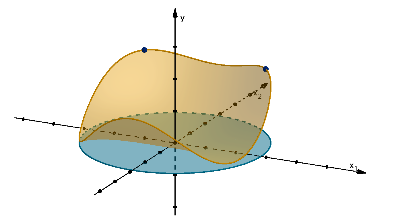
Figure 4.14: The maximizers of y = x

+ x

+ 2x

subject to 8 − x

− x

≥ 0

Main Ideas

The algebraic expressions tell us when the objective function is continuous and the feasible set is

closed.

Draw the feasible set to decide whether it is bounded.

If the EVT applies, we can evaluate f at all of the points that passed our necessary conditions.

The one that attains the greatest value is the maximizer.

171

4.1.3

Section Summary

The most important deﬁnitions and results from this section were

The extreme value theorem (Theorem 4.1)

The meaning of closed and bounded (Deﬁnition 4.2)

Level sets, upper level sets, and their intersections are closed (Theorems 4.3 and 4.4)

172

4.2

The Bordered Hessian

Goals:

1 Use the bordered Hessian to identify local maximizers of a function subject to a constraint.

4.2.1

The Bordered Hessian

We used the Hessian matrix to recognize maximizers and minimizers in unconstrained optimization.

This worked because the Hessian computed the second derivative over a straight line a+ tv. An equality

constraint does not usually contain straight lines. The test for the second derivative will need to take

account of the shape of the level set g(x) = 0.

Deﬁnition 4.5

Given a constrained optimization problem with Hessian L, the matrix HL(λ, x) is called the bordered

Hessian of the constrained optimization problem.

Example

The 2-variable bordered Hessian has the form

HL(λ, x

, x

) =





λλ

λ1

λ2

λ1









0 g

+ λg





Why is this called “bordered?”

The bottom right 2 × 2 minor looks like a Hessian.

It is bordered to the left and above by ∇g.

Notice that we have switched the order of variables in our Lagrangian. This is common when writing

the bordered Hessian. Placing the border on the top allows us to write our condition for a local maximizer

in a familiar way. If we instead prioritized consistency, we could keep the λ last and modify our condition.

173

4.2.1 The Bordered Hessian

Theorem 4.6

Let f(x) be an n-variable function and g(x) = 0 be a constraint. If (ℓ,a) satisﬁes the ﬁrst-order

condition of the Lagrangian and the upper left square minors of HL(ℓ,a) satisfy

(−1)

| < 0 2 ≤ i ≤ n + 1,

then a is a strict local maximizer of f among points on the constraint.

Remark

We do not test |M

|, since M

= [0].

We generally do not need to worry about M

either, since

| =



0 g

+ λg



= −(g

)

Notice the inequality is reversed from the unconstrained second-order condition.

Variant of Theorem 4.6

Let f(x) be an n-variable function and g(x) = 0 be a constraint. If (ℓ,a) satisﬁes the ﬁrst-order

condition of the Lagrangian and the upper left square minors of HL(ℓ,a) satisfy

| < 0 2 ≤ i ≤ n + 1,

then a is a strict local minimizer of f among points on the constraint.

Remark

We might hope to quickly extend this to a global condition, but unfortunately, HL only tells us about

the second derivatives at a critical point. Deriving a condition that works for all points on the constraint

is possible but more complicated.

174

4.2.2

Using the Bordered Hessian

Let f(x

, x

) = x

+ x

on the domain

D = {(x

, x

) : x

> 0, x

> 0}

Find the critical point of f on the constraint x

+ x

= 2. Classify it as a local maximizer or local

maximizer of f (or neither) on the constraint.

Solution

The Lagrangian is

L(x

, x

, λ) = x

+ x

+ λ(2 − x

− x

)

Here are the ﬁrst-order conditions. We can solve them, using the fact that x

> 0 and x

> 0.

− 4λx

= 0 2x

− 4λx

= 0 2 − x

− x

= 0

2λ

= x

2 − x

− x

= 0

2 = 2x

1 = x

1 =

2λ

λ =

The critical point is



1, 1,



. Switching the order of the variables, we compute

HL(λ, x

, x

) =





0 −4x

−4x

2 − 12λx

−4x

0 2 − 12λx







, 1, 1







0 −4 −4

−4 −4 0

−4 0 −4





The determinants of the upper left square minors are

| =



0 −4

−4 −4



= −16

| =



0 −4 −4

−4 −4 0

−4 0 −4



= 0 + 4



−4 0

−4 −4



− 4



−4 −4

−4 0



= 128

175

4.2.2

Using the Bordered Hessian

(−1)

(−16) < 0 and (−1)

(128) < 0. According to Theorem 4.6, (1, 1) is a strict local maximizer.

∇f(1, 1)

Figure 4.15: The level sets of x

+ x

and the constraint x

+ x

= 2

4.2.3

The Multi-Constraint Bordered Hessian

For more variables, the test requires more determinants.

Theorem 4.7

Let f (x) be an n-variable function and {g

(x) = 0} be a set of m constraint equations. If (



ℓ,a) satisﬁes

the ﬁrst-order condition of the Lagrangian and the upper left square minors of HL(



ℓ,a) satisfy

(−1)

| < 0 2m ≤ i ≤ n + m,

then a is a strict local maximizer of f(x) among the feasible points.

176

4.2.4

The Bordered Hessian and Inequality Constraints

If we combine the determinant of the bordered Hessian with the requirement that ℓ > 0, then we can

guarantee that f(x) < f(a) on the equality constraint and in the direction of ∇g(a) from the equality

constraint. This guarantees a neighborhood of some size in which a is a maximizer among feasible

points.

4.2.5

Section Summary

The most important deﬁnitions and results from this section were

The deﬁnition of the bordered Hessian (Deﬁnition 4.5)

The bordered Hessian determinant test for a maximizer (Theorems 4.6)

177

4.3

Separation

Goals:

1 Use normal vectors to describe half-spaces of a hyperplane.

2 Apply optimization by separation arguments.

4.3.1

Upper Level Sets and Optimization

Recall our necessary conditions for a maximizer of f(x) subject to g(x) ≥ 0. If the constraint is

binding, we learned to check that ∇f(a) is parallel to ∇g(a), meaning the level sets are parallel. We

also check that λ ≥ 0, meaning that ∇f(a) points away from the feasible set. However, these checks

are not suﬃcient. We will construct an example that passes these conditions but isn’t a maximizer.

Recall the following deﬁnition

Deﬁnition 2.13

The upper level sets of a function f(x) with domain D are the sets

{x ∈ D | f(x) ≥ c} for some number c

The lower level sets are

{x ∈ D | f(x) ≤ c} for some number c

The following characterization will be important to our arguments.

Lemma 2.14

Suppose ∇f(x) =



0, and x(t) is a path that passes through a in the level set f(x) = c at t

If x

′

) makes an acute angle with ∇f (a), then x(t) travels into the upper level set f (x) ≥ c.

If x

′

) makes an obtuse angle with ∇f (a), then x(t) travels into the lower level set f (x) ≤ c.

178

Consider the following diagram of a feasible set and an upper level set. The point a satisﬁes

∇f(a) = −λ∇g(a) and λ ≥ 0, but we can see that there are also feasible points in the interior of the

upper level set, like



b. f(



b) may be greater than f (a).

∇f(a)

∇g(a)

a



Figure 4.16: An upper level set and feasible set for which a is not a maximizer

We would like a condition to rule out this behavior. Suppose that a line separates the upper level

set f(x) ≥ c from the feasible set. This prevents any higher values of f from appearing in the feasible

set.

a

Figure 4.17: The upper level set of f, a feasible set, and a separating line

4.3.2

Hyperplanes and Half-Spaces

To formalize this reasoning, we ﬁrst present the notation for a separating line and generalize it to

higher dimensions. Every line h in R

has a normal vector v. h divides R

into two half-planes:

on the side of v

−

on the other side.

179

4.3.2

Hyperplanes and Half-Spaces

−

v

a

Figure 4.18: A line, its normal vector v, and its half spaces

For any point x, the vector that points from a to x is

x −a.

The angle of this vector with v tells us which half-plane contains x. The dot product tells us whether

this angle is acute, obtuse or right.

Lemma 4.8

Suppose h is a line in R

with normal vector v, and a is a point on h. For any point x

v · (x −a)











> 0 if x lies in h

= 0 if x lies on h

< 0 if x lies in h

−

Figure 4.19: The angle between a vector and the normal vector of a line

180

The analogous object in R

is a plane h. It has a normal vector and divides R

into two half-spaces

and h

−

. The sign of v · (x −a) tests which half-space x lies in. Speciﬁcally, x lies on the plane, if

v · (x −a) = 0.

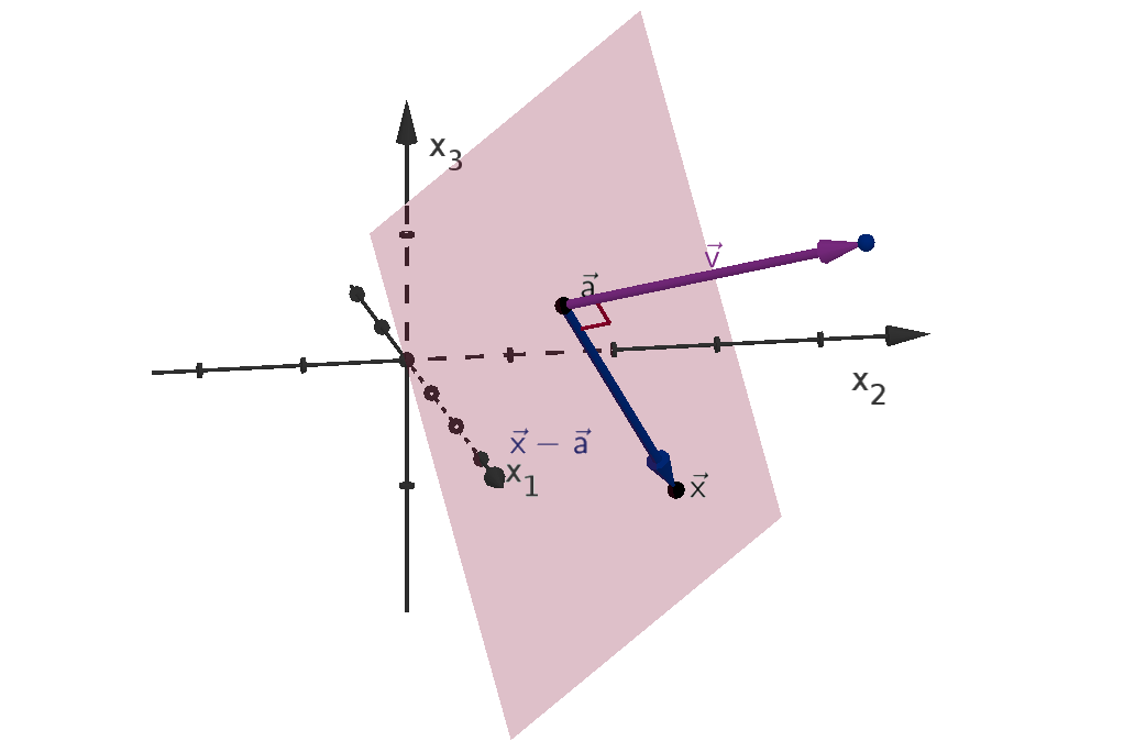
Figure 4.20: A plane, its normal vector v, and a vector on it

This reasoning works in any dimension to deﬁne a set of points whose displacement from a known

point a is orthogonal to a normal vector v.

Deﬁnition 4.9

In R

, v · (x −a) = 0 deﬁnes a line.

In R

, v · (x −a) = 0 deﬁnes a plane.

In R

, v · (x −a) = 0 deﬁnes a hyperplane, a linear (n − 1)-dimensional subspace.

When dimension is general or ambiguous, we use the term hyperplane as a catch-all term. We can

rewrite our dot product lemma to reﬂect the n-dimensional case.

Variant of Lemma 4.8

Suppose h is a hyperplane with normal vector v and a is a point on h. For any point x

v · (x −a)











> 0 if x lies in h

= 0 if x lies on h

< 0 if x lies in h

−

181

4.3.2

Hyperplanes and Half-Spaces

For a more concise test, we can let k = v ·a. We can rewrite our dot product

v · (x −a) = v · x −v ·a = v · x − k

and the lemma

v ·x











> k if x lies in h

= k if x lies on h

< k if x lies in h

−

4.3.3

Optimization by Separation

In Figure 4.17, a line separates the upper level set of f and the feasible set. The point where they

meet appears to be a maximizer of f. We now have the notation to formalize this argument.

Theorem 4.10

Suppose we have a continuous objective function f(x) and some constraint(s). Suppose x

∗

is in the

feasible set and let f(x

∗

) = c. If there is a hyperplane h such that

1 the upper level set f(x) ≥ c has no points in h

−

2 the feasible set has no points in h

then x

∗

is a maximizer of f(x) subject to the constraint(s).

This method is called optimization by separation and h is a separating hyperplane. It is a

suﬃcient condition, but it requires us to know the proper hyperplane h.

Notice both the upper level set and the feasible set may contain have points on h. In fact, x

∗

one of them. What if they share an additional point a in h? a must lie on the boundary of the upper

level set, arbitrarily close to points for which f(x) < c. Since f(x) is continuous, f(a) = c. We can still

conclude that x

∗

is a maximizer, but not a unique maximizer.

182

a



Figure 4.21: An upper level set of f and the feasible set intersecting multiple times along their

separating line

We can modify this theorem by stipulating that x

∗

is either

1 the only point of the upper level set on h or

2 the only feasible point on h.

In this case we can conclude that x

∗

is the unique maximizer.

If we want to avoid talking directly about the hyperplane h, we can think of v ·x as a function of x.

Its level sets are the hyperplanes v ·x = k. The value of v ·x increases as we travel in the direction of v.

k > k< k

v

x

∗

Figure 4.22: Some level sets of v ·x that intersect an upper level set of f and a feasible set

Our separation argument can be rephrased to require that the upper level set meets only higher

values of v ·x while the feasible set meets only lower values of v · x. We can verify this algebraically.

Suppose x be a point in the upper level set of f(x). Lemma 4.8 states that x does not lie in h

−

, if

v · (x − x

∗

) ≥ 0

v ·x ≥ v · x

∗

183

4.3.3 Optimization by Separation

This inequality indicates that the value of v · x at x

∗

is less than or equal to the value at any other

point in the upper level set. In other words, x

∗

minimizes the function v · x subject to the constraint

f(x) ≥ c.

To show that the feasible set has no points in h

we can check that for each feasible x:

v · (x − x

∗

) ≤ 0

v ·x ≤ v · x

∗

This means that the value of v · x at x

∗

is greater than or equal to the value at any other x in the

feasible set. In other words, x

∗

maximizes the function v · x subject to the constraints of the original

optimization problem. We can restate Theorem 4.10 in terms of this new vocabulary.

Alternate Formulation of Theorem 4.10

Suppose we have a continuous objective function f and some constraints. If f(x

∗

) = c and for some

v =



0 we have

1 x

∗

minimizes v ·x subject to f(x) ≥ c

2 x

∗

maximizes v ·x subject to the constraints

Then x

∗

maximizes f(x) given the constraints.

We can see that this is a condition for a maximizer without knowing much about hyperplanes. If

the feasible points all have values of v ·x less than or equal to k and the upper level sets all have values

greater than or equal to k, then the feasible set and the upper level can only meet where v · x = k.

4.3.4

The Tangent Hyperplane

An observant reader will have noticed that our separating lines have always been tangent to the level

curve f(x) = c. This is not a coincidence. It occurs in higher dimensions as well, where the tangent

lines become tangent hyperplanes.

Deﬁnition 4.11

Suppose a point a lies on level set f (x) = c, and ∇f(a) =



0. The tangent hyperplane to f(x) = c

at a is the hyperplane containing of all the tangent lines to f (x) = c at a. Its normal vector is ∇f(a).

Its equation is

∇f(a) · (x −a) = 0

184

If ∇f(a) = 0, the only candidate for a separating hyperplane is the tangent hyperplane to f(x) = c.

Any other hyperplane would contain some vector w such that ∇f(a) · w > 0, meaning it would cut into

the upper level set of f at a.

On the other hand, we have seen examples where a tangent line fails to keep the upper level set out

of h

−

∇f(a)

a

Figure 4.23: An upper level set that crosses its own tangent line

For this reason, optimization by separation is only realistic for functions with nicely shaped level sets.

We will discover a class of such functions in the next section.

4.3.5

Section Summary

The most important deﬁnitions and results from this section were

Hyperplanes and the dot product test (Deﬁnition 4.9 and Lemma 4.8)

Optimization by separation, both formulations (Theorem 4.10 and its variant)

Equation of a tangent hyperplane to a level set (Deﬁnition 4.11)

185

4.4

Concave Programming

Goals:

1 Understand the geometric consequences of concavity on constrained optimizations.

2 Apply suﬃcient conditions for maximizers of concave functions with concave constraints.

4.4.1

Kuhn-Tucker Suﬃciency

When is a separation argument possible? When does the tangent hyperplane separate the upper level

set from the feasible set? Concavity is one way to guarantee this. There is an a rich theory and toolset

for optimization that is speciﬁc to concave functions. This is the ﬁeld of concave programming. Here

is our main result.

Theorem 4.12

Given an objective function f(x) and constraints g

(x) ≥ 0, suppose (x

∗



∗

) satisﬁes the Kuhn-Tucker

conditions:

(x

∗



∗

) = 0 for all i

(x

∗

) ≥ 0 and λ

∗

≥ 0 with complementary slackness for each j

If f(x) and the g

(x) are all concave functions, then x

∗

maximizes f(x), subject to the constraints.

It is worth understanding the full argument of this theorem that follows, but the essential ideas are:

1 The upper level sets of a concave function are convex sets. This applies not only to f (x) ≥ c but

also to the feasible set, which is an intersection of the upper level sets: g

(x) ≥ 0.

2 Using this convexity, we can show that the tangent hyperplane to f(x) = c separates the upper

level set f(x) ≥ c from the feasible set.

186

∇f(x

∗

)

Figure 4.24: A feasible region deﬁned by multiple concave inequalities separated from the upper level

set of f by a tangent line

Remark

This suﬃcient condition is especially powerful because once we ﬁnd a point that satisﬁes Kuhn-Tucker,

we can stop looking. If, by luck or cleverness, we ﬁnd a solution in the ﬁrst case of complementary

slackness we try, then we have found the maximizer. We need not examine the other cases at all.

4.4.2

Applying the Kuhn-Tucker Suﬃcient Condition

Find the maximum value of f(x

, x

) = 4x

+ x

on the region

S = {(x

, x

) : 25 − 7x

− x

≥ 0, x

+ x

− 5 ≥ 0, and 25 − x

− x

≥ 0}

+ x

− 5 = 0

25 − x

− x

= 0

25 − 7x

− x

= 0

Figure 4.25: The feasible set S

187

4.4.2

Applying the Kuhn-Tucker Suﬃcient Condition

Solution

Increasing x

seems to be the most important factor in increasing f , but larger x

helps too. We should

draw and examine the region S. The set x

+ x

−5 ≥ 0 appears to be nonconvex. On the other hand,

based on our diagram, that inequality appears not to bind. We will instead maximize f over the region

T = {(x

, x

) : 25 − 7x

− x

≥ 0, x

≥ 0, and 25 − x

− x

≥ 0}

S is a subset of T so a maximizer in T that lies in S is a maximizer in S. This modiﬁed problem has

the following Lagrangian:

L(x

, x

, λ

) = 4x

+ x

+ λ

(25 − 7x

− x

) + λ

+ λ

(25 − x

− x

The Kuhn-Tucker conditions are

= 4 − 7λ

− 2λ3x

= 0

= 1 − λ

+ λ

− 2λ

25 − 7x

− x

≥ 0 λ

(25 − 7x

− x

) = 0

≥ 0 λ

= 0

25 − x

− x

≥ 0 λ

(25 − x

− x

) = 0

We might guess that 25 −7x

−x

= 0 and 25−x

−x

= 0 are binding at the maximizer and x

≥ 0 is

not. Based on that guess, we ﬁrst consider the case where λ

= 0. Next we use the binding constraints

to solve for x

and x

25 − 7x

− x

= 0 25 − x

− x

= 0

25 − 7x

= x

25 − x

− (25 − 7x

)

= 0

25 − x

− 49x

+ 350x

− 625 = 0

−50x

+ 350x

− 600 = 0

−50(x

− 3)(x

− 4) = 0

= 3 or 4

25 − 7(3) = 4 = x

25 − 7(4) = −3 = x

We can look ahead and see that x

= −3 will not satisfy our inequalities, so we set (x

, x

) = (3, 4).

We use the remaining equations to solve for the λ

and λ

4 − 7λ

− 2λ

= 0 1 − λ

− 2λ

= 0

4 − 7λ

− 6λ

= 0 1 − λ

− 8λ

= 0

1 − 8λ

= λ

4 − 7 + 56λ

− 6λ

= 0

50λ

= 3

1 −

= λ

188

Our solution is



3, 4,

, 0,



. We check, and it satisﬁes the remaining inequalities.

≥ 0

= 4 ≥ 0

≥ 0

There are 7 other cases of complementary slackness to check, but we can avoid them. Our suﬃciency

theorem applies to (3, 4). We only need to check for concavity of the relevant functions.

+ x

is concave because it is linear.

25 − 7x

− x

is concave because it is linear.

25 −x

−x

is strictly concave because its hessian is



−2 0

0 −2



, which is negative deﬁnite for

all (x

, x

We ignored the constraint x

+ x

− 5 ≥ 0.

Based on these checks, the theorem applies, and (3, 4) must be a maximizer of f on T . Since (3, 4)

satisﬁes

+ x

− 5 = 4 + 9 − 5 ≥ 0

it lies in S as well. Since S ⊆ T , we conclude (3, 4) is also a maximizer of f in S. The maximum value

is f(3, 4) = 4(3) + (4) = 16.

Main Idea

The most common methods to check concavity are

linear functions are concave

functions with negative deﬁnite Hessians are strictly concave

If the functions are concave, and we guess the right combination of binding constraints, then we only

need to check the Kuhn-Tucker conditions for that case.

189

4.4.2

Applying the Kuhn-Tucker Suﬃcient Condition

Remark

The underlying separation argument was between the convex upper level set f(x

, x

) ≥ 16 and the

convex set

T = {(x

, x

) : 25 − 7x

− x

≥ 0, x

≥ 0 and 25 − x

− x

≥ 0}

Since (3, 4) is a maximizer on T , it is a maximizer on S.

∇f(3, 4)

Figure 4.26: A convex set T containing S, an upper level set, and a separating line

The reasoning of this example also suggests the following variant.

Variant of Theorem 4.12

Given an objective function f(x) and constraints g

(x) ≥ 0, suppose (x

∗



∗

) satisﬁes the Kuhn-Tucker

conditions.

If f(x) and the binding g

(x) are all concave, then x

∗

maximizes f(x), subject to the constraints.

4.4.3

Proving Kuhn-Tucker Suﬃciency

This will be an extensive argument with many parts, but there are two reasons to give it our attention.

1 Some of the lemmas along the way are useful or interesting in their own right.

2 There are many ways to modify this argument for diﬀerent circumstances. If you understand the

original argument, you can understand or even generate these variants.

190

Our ﬁrst step is to understand the upper level sets of concave functions.

Lemma 4.13

If f(x) is a concave function, then the upper level set f(x) ≥ c is a convex set.

We can argue this directly from the deﬁnition of an upper level set, the deﬁnition of a convex set,

and the following inequality for concave functions:

f((1 − t)a + t



b) ≥ (1 − t)f(a) + tf(



b).

Figure 4.27: The segment from a to



b in the upper level set of f(x)

Proof

Let a and



b be points in the upper level set f(x) ≥ c. We will show that the segment between a and



also lies in this upper level set. The points on the segment from a to



b are parametrized by

(1 − t)a + t



b 0 ≤ t ≤ 1

If we evaluate f along these points we get

f((1 − t)a + t



b) ≥ (1 − t)f(a) + tf(



b) (f is concave)

≥ (1 − t)c + tc (a and



b lie in the upper level set)

≥ c

Since f((1 −t)a + t



b) ≥ c, (1 −t)a + t



b lies in the upper level set. Since this is true for every t between

0 and 1, the entire segment from a to



b lies in the upper level set. Since this is true for all a and



b in

the upper level set, we conclude that the upper level set is convex.

191

4.4.3 Proving Kuhn-Tucker Suﬃciency

We now know that if f is concave, then its upper level sets are convex. For a separation argument,

we also would like to know they do not cross their tangent hyperplane. Fortunately, this is the case.

Lemma 4.14

Let

f(x) be a continuously diﬀerentiable function

a be a point such that f(a) = c and ∇f (a) =



h be the tangent hyperplane to f(x) = c at a.

If upper level set f(x) ≥ c is convex, then it does not intersect h

−

Proof

Suppose



b is any point in the upper level set f(x) ≥ c. We want to show that



b does not lie in h

−

Since the upper level set is convex, the entire segment

x(t) = (1 − t)a + t



b 0 ≤ t ≤ 1

= a + t(



b −a)

must lie within it. This speciﬁcally requires that the direction vector x

′

(0) =



b −a points into the upper

level set at a. Lemma 2.14 tells us that if ∇f(a) · x

′

(0) < 0, then x(t) travels into the lower level set.

Thus ∇f · (



b −a) ≥ 0. By Lemma 4.8,



b does not lie in h

−

∇f(a)

a



Figure 4.28: The vector



b −a in a

convex upper level set making an acute

angle with ∇f(a)

∇f(a)

a



Figure 4.29: The vector



b −a leaving an

upper level set and making an obtuse

angle with ∇f(a)

Now we turn our attention to the constraint functions. Lemma 4.13 applies as well to each g

as it

does to f. If each function g

(x) is concave, then each upper level set g

(x) ≥ 0 is convex. With some

very familiar looking conditions on ∇g

(a), we can ensure that the feasible set stays on one side of the

tangent hyperplane to f(x) = c.

192

Corollary 4.15

Let f(a) = c and ∇f(a) =



0. Let h be the tangent hyperplane to f(x) = c at a. If

1 The upper level sets g

(x) ≥ 0 are convex

2 ∇f(a) = −

∇g

(a) for some numbers λ

3 For each j, λ

≥ 0 if g

(a) = 0 and λ

= 0 otherwise

then the intersection of the upper level sets g

(x) ≥ 0 does not intersect h

The geometry is easiest to visualize if we consider a single constraint g(x) ≥ 0. In this case,

∇f(a) = −λ∇g(a). For any



b in g(x) ≥ 0, the vector



b −a makes an acute angle with ∇g(a). Thus it

makes an obtuse angle with ∇f (a), meaning



b lies in h

−

∇f(a)

∇g(a)

a



Figure 4.30: The vector



b −a in a convex feasible set making an obtuse angle with ∇f(a)

For multiple constraints, angles are too diﬃcult to discern. The dot product provides a cleaner

argument.

Proof

Let



b be a point in the intersection of the upper level sets. For each g

(x) that is binding at a, we can

apply Lemma 4.14 to the convex upper level set g

(x) ≥ 0. As that proof argued, we can conclude that

∇g

· (



b −a) ≥ 0.

By Lemma 4.8, the sign of ∇f (a) · (



b −a) will tell us whether



b lies in h

. We can substitute as

193

4.4.3 Proving Kuhn-Tucker Suﬃciency

follows:

∇f(a) · (



b −a) = −





∇g

(a)





· (



b −a)

= −

∇g

(a) · (



b −a)

We can determine the sign of each term of the summation.

1 For nonbinding g

, λ

= 0.

2 For binding g

, λ

≥ 0 and ∇g

(a) · (



b −a) ≥ 0.

We conclude that ∇f (a) · (



b −a) ≤ 0. Thus



b does not lie in h

We now have the ingredients to prove Theorem 4.12. There are two cases of complementary slackness

to consider when proving this theorem.

1 If all λ

∗

= 0 then ∇f(x

∗

) = 0. Since f is concave, a variant of Corollary 1.23 tells us that x

∗

an unconstrained maximizer of f. Corollary 2.2 tells us that since it lies in the feasible set, is also

a maximizer there.

2 If some λ

∗

> 0 then we can put together the results of this section to conclude the upper level

set of f and the feasible set lie on opposite sides of h. This is the requirement for optimization

by separation established in Theorem 4.10, so x

∗

is a maximizer.

Here is a diagram containing the reasoning for each case.

binding λ

∗

> 0

all λ

∗

= 0

∇f(x

∗

) =



f(x) is

concave

f(x) ≥ c is convex

f(x) ≥ c does not

intersect h

−

(x) are

concave

(x) ≥ 0

are convex

∇f(x

∗

) = −

∗

∇g

(x

∗

)

feasible set does

not intersect h

x

∗

is a max

x

∗

is a max

in the feasible set

Lem 4.13

Lem 4.14

Lem 4.13

Cor 4.15

Thm 4.10

Cor 1.38

Cor 2.2

194

4.4.4

Variants of Kuhn-Tucker Suﬃciency

In a separation argument, the upper level set and the feasible set may meet at many points in h. For

example, we could have an entire line segment of intersection, and every point on that segment would

satisfy Kuhn-Tucker.

∇f(x

∗

)

Figure 4.31: An upper level set of f and the feasible set intersecting along a separating line

This pathology only exists if both sets contain multiple points on the separating hyperplane. If one

of the sets is strictly convex, this will not happen. We can achieve this with strict concavity. Each

lemmas we used has a variant for strict concavity.

Variant of Lemma 4.13

If f(x) is a strictly concave function then the upper level set f(x) ≥ c is strictly convex.

Variant of Lemma 4.14

Suppose we have

a continuously diﬀerentiable function f(x)

a point a such that f(a) = c and ∇f (a) =



the tangent hyperplane to f(x) = c at a, denoted h.

If upper level set f(x) ≥ c is strictly convex, then it lies entirely within h

, except for the point a.

195

4.4.4 Variants of Kuhn-Tucker Suﬃciency

Variant of Corollary 4.15

Let f(a) = c and ∇f(a) =



0. Let h be the tangent hyperplane to f(x) = c at a. If

1 The upper level sets g

(x) ≥ 0 are strictly convex

2 ∇f(a) = −

∇g

(a) for some numbers λ

3 For each j, λ

≥ 0 if g

(a) = 0 and λ

= 0 otherwise

then the intersection of the upper level sets g

(x) ≥ 0 lies entirely within h

−

except the point a.

We can use these lemmas to guarantee a unique maximizer. We can either keep the upper level set

or the feasible set from having multiple points on h.

Theorem 4.12 for a Unique Maximizer

Given an objective function f(x) and constraints g

(x) ≥ 0, suppose (x

∗



∗

) satisﬁes the Kuhn-Tucker

conditions. If f(x) and the binding g

(x) are concave, and additionally either

1 f(x) is strictly concave, or

2 at least one constraint binds and the binding g

(x) are strictly concave,

then x

∗

is the unique maximizer of f(x), subject to the constraints.

Another avenue of modiﬁcation is to include equality constraints. One method is to treat the equality

constraint as an inequality constraint. The level set is a subset of the upper level set. By Corollary 2.2,

a maximizer over an inequality constraint that happens to bind is also a maximizer over the equality

constraint. This requires the constraint function to be concave and its λ

to be positive.

Alternately, if the equality constraint is linear, then its level set is a hyperplane, which is convex.

Thus the feasible set is still convex. Corollary 4.15 still holds regardless of the sign of λ

, because

∇g

(a) · (



b −a) = 0. We can formalize this possibility with the following variant.

Theorem 4.12 with Equality Constraints

Given an objective function f (x) and constraints of the forms g

(x) ≥ 0 and g

(x) = 0, suppose (x

∗



∗

)

satisﬁes the Kuhn-Tucker conditions.

If f(x) and the binding g

(x) are all concave, and the equality constraints are linear, then x

∗

maximizes f(x), given the constraints.

196

This section contains just a few possibilities. There are other ways to modify our suﬃciency theorems

that allow them to apply in more situations or to draw stronger conclusions.

4.4.5

Slater’s Condition

Concavity has produced a convenient suﬃcient condition for constrained optimization. It can also

help simplify our necessary conditions. Recall that the Kuhn-Tucker conditions are a necessary condition,

but they have an exception. Theorem 2.23 states that a maximizer a must either satisfy the Kuhn-Tucker

conditions or have binding ∇g

(a) that are linearly dependent.

Checking for linearly dependent gradient vectors is diﬃcult, especially if we do not know where to

look for them. Slater’s condition allows us to skip that check in some situations.

Slater’s condition requires that the objective and constraint functions are concave. It also requires

the feasible set to have an interior, rather than collapsing to a lower dimensional set. Formally, it

demands the existence of a point



b in the interior. This point is not special. If the feasible region has

an interior, then you can identify inﬁnitely many points inside it by looking at a diagram.

Theorem 4.16 [Slater’s Condition]

Suppose that the functions f(x) and g

(x) satisfy Slater’s condition:

1 f(x) and the g

(x) are all concave functions

2 there is at least one point



b in the interior of the feasible set, meaning

(



b) > 0 for all j

If a is a local maximizer of f(x) subject to g

(x) ≥ 0, then a satisﬁes the Kuhn-Tucker conditions.

Remark

Slater’s condition checks for concavity, just like Theorem 4.12 (our suﬃcient condition). This means

that if f(x) and g

(x) satisfy Slater’s condition, then the Kuhn-Tucker conditions are both necessary

and suﬃcient for a maximizer.

Slater’s condition doesn’t prevent the gradient vectors of the binding g

from being linearly depen-

dent. Instead it argues that even if the gradient vectors are linearly dependent at a, the Kuhn-Tucker

conditions must still be satisﬁed in order for a to be a maximizer.

Slater’s condition can be strengthened to handle equality constraints in the case that those are linear.

197

4.4.5 Slater’s Condition

Variant of Theorem 4.16

Suppose that we are maximizing f(x) subject to constraints of the form g

(x) ≥ 0 or g

(x) = 0.

Suppose further that

1 f(x) and the inequality constraint functions g

(x) are concave

2 the equality constraint functions g

(x) are linear

3 there is at least one point



b in the relative interior of the feasible set, meaning

(



b) > 0 for all inequality constraints

(



b) = 0 for all equality constraints

If a is a local maximizer, then it satisﬁes the Kuhn-Tucker conditions.

4.4.6

The Separating Hyperplane Theorem

Throughout this section, we have used tangent hyperplanes to separate convex sets. It is possible to

make these arguments without separation, however. Here is a short alternative proof of Theorem 4.12.

Proof

x

∗

satisﬁes the ﬁrst-order condition of a stubborn lagrangian, in which



λ is held constant at



∗

(x) = f(x) +

∗

(x)

Since λ

∗

≥ 0, L

∗

is a sum of concave functions. By Theorem 1.20, L

∗

is concave. Thus x

∗

is a

maximizer of L

∗

. x

∗

also satisﬁes λ

∗

(x

∗

) = 0 by complementary slackness. If we compare x

∗

and

any other feasible point a, we have

∗

(x

∗

) ≥ L

∗

(a)

f(x

∗

) +

∗

(x

∗

) ≥ f(a) +

∗

(a)

f(x

∗

) + 0 ≥ f(a) +

∗

|{z}

≥0

(a)

|{z}

≥0

f(x

∗

) ≥ f(a)

Since this holds for any feasible a, we can conclude that x

∗

is a maximizer of f(x) subject to g

(x) ≥ 0.

198

This argument does not establish a separating hyperplane, even though we know one exists from our

longer proof. It turns out that in any successful maximization argument for a concave function over a

convex feasible set, the hyperplane is there, whether we use it or not. The following famous theorem

guarantees that.

Theorem 4.17 [The Separating Hyperplane Theorem]

If S and U are two convex sets, at least one has a non-empty interior, and they share no interior points

in common, then there is a vector v and a number k such that

1 For all x in U, v · x ≥ k

2 For all x in S, v ·x ≤ k

Remark

This theorem tells us that if a convex upper level set U and a convex feasible set S meet only at their

boundaries, then the hyperplane v · x = k separates them. It does not tell us what v is or how to

construct it.

As you might infer from this remark, the applications of the separating hyperplane theorem tend to

be abstract. The proof requires ideas from analysis.

4.4.7

Section Summary

The most important deﬁnitions and results from this section were

Upper level sets of concave functions are convex (Lemma 4.13)

Convex upper level sets lie in one half space of their tangent hyperplanes (Lemma 4.14)

Kuhn-Tucker suﬃciency for concave functions (Theorem 4.12)

Slater’s condition (Theorem 4.16)

This is also a good time to summarize the suﬃcient conditions we have covered. They diﬀer in when

they can be applied and what conclusion they draw.

199

4.4.7

Section Summary

Suﬃcient Conditions for Constrained Optimization

Condition Limited to Conclusion

EVT bounded sets one of the critical points

is a maximizer

Bordered Hessian binding constraint this critical point

is a local maximizer

KT Suﬃciency concave functions this critical point

is a maximizer

200

4.5

Quasiconcavity

Goals:

1 Recognize a quasiconcave function from its graph or level sets

2 Apply quasiconcavity in suﬃcient conditions for a maximizer

3 Use concavity and nondecreasing compositions to test for quasiconcavity

4 Use a determinant test to verify quasiconcavity

4.5.1

Limitations of Concave Programming

Concave programming provided suﬃcient conditions for a maximizer on one or more constraints.

Our argument excluded functions with badly behaved level sets in order to guarantee separation, but

did it exclude too many?

The function f(x) =

−2x+2

has convex upper level sets, but it is not a concave function. Could

we make a separation argument for it?

Figure 4.32: The graph of y =

−2x+2

and a convex upper level set

Another example: f (x

, x

) = x

(restricted to x

, x

> 0) has strictly convex upper level sets.

It is not a concave function, because

Hf (x

, x

) =



0 1

1 0



201

4.5.1 Limitations of Concave Programming

∇f(x

, x

)

Figure 4.33: Several level sets and one upper level set of f(x

, x

) = x

4.5.2

Quasiconcave Functions

Theorem 4.12 requires that the objective function and constraint functions are concave, but the only

part of the proof that used their concavity was the ﬁrst step: that concave functions have convex upper

level sets. We have now seen examples of other functions that have this property. These examples

belong to a broader class of functions, on which the main ideas of concave programming still apply. We

call them quasiconcave.

Deﬁnition 4.18

A function f(x) is quasiconcave if for any points a and



b in the domain of f(x),

f((1 − t)a + t



b) ≥ min{f(a), f(



b)} for all 0 ≤ t ≤ 1

It is quasiconvex if

f((1 − t)a + t



b) ≤ max{f(a), f(



b)} for all 0 ≤ t ≤ 1

Quasiconcavity is a statement about the height of the graph over a path that goes across and then

up.

f((1 − t)a + t



| {z }

line from a to



) ≥ min{f(a), f(



b)}

| {z }

horizontal line

for all 0 ≤ t ≤ 1

202

Figure 4.34: The graph of a quasiconcave function and the across and up path

Remark

“Across and up” is designed so that the path has a height that is the minimum of f(a) and f(



b) for

each x between them. If it lies below the graph then

f((1 − t)a + t



b) ≥ min{f(a), f(



b)} for all 0 ≤ t ≤ 1.

Do not make an “across and down” or “up and across” path by mistake. Those will test a diﬀerent

inequality.

The name quasiconcavity suggests that these functions should be similar to concave functions. In

fact, concavity is a stronger condition than quasiconcavity. A visual argument is best here. Theorem

1.19 showed that a function is concave, if and only if its graph lies above its secants.

The across and up path lies below the secant from (a, f(a)) to (



b, f(



b)). If y = f(x) lies above the

secant, then it also lies above the across and up path.

Theorem 4.19

If f(x) is a concave function, then it is also a quasiconcave function.

203

4.5.2

Quasiconcave Functions

Figure 4.35: The secant and the across and up path below y = f (x)

Quasiconcavity is easiest to recognize in single-variable functions. We can verify that across and up

paths stay below the graph y = f(x) for functions with the following shapes.

Lemma 4.20

Suppose f(x) is a one-variable function. f (x) is quasiconcave, if one of the following is true about

f(x):

1 f(x) is non-decreasing.

2 f(x) is non-increasing.

3 For some a, f(x) is non-decreasing before a and nonincreasing after a.

Functions that satisfy 1 or 2 are called monotone.

Remark

These conclusions only make sense for single-variable functions. Increasing and decreasing are not words

that describe multivariable functions.

204

Figure 4.36: The across and up path below a non-increasing y = f (x)

Our goal in deﬁning quasiconcavity was to produce a large class of functions whose upper level sets

allowed for separation arguments. In fact, the quasiconcave functions are the broadest possible such

class. Every function with convex upper level sets is quasiconcave, and every quasiconcave function has

convex upper level sets.

Lemma 4.21

f(x) is a quasiconcave function, if and only if every upper level set f(x) ≥ c is a convex set.

Figure 4.37: The segment from a to



b in the upper level set of f(x)

The proof relies on combining the deﬁnitions of quasiconcavity, upper level sets, and convex sets.

205

4.5.2

Quasiconcave Functions

Proof

There are two directions of argument that we need to make.

1 Suppose that f (x) is quasiconcave. Let a and



b be in the upper level set f(x) ≥ c. By deﬁnition,

we know that f(a) ≥ c and f(



b) ≥ c. The points on the segment from a to



b are parametrized by

(1 − t)a + t



b 0 ≤ t ≤ 1

If we evaluate f along these points we get

f((1 − t)a + t



b) ≥ min{f(a), f(



b)} (f is quasiconcave)

≥ c (a and



b lie in the upper level set)

Thus the segment lies in the upper level set f(x) ≥ c. Since this holds for any a and



b in any

upper level set, we conclude that every upper level set of f(x) is convex.

2 Now suppose that every upper level set of (x) is convex. Let a and



b be any points in the domain.

Let c = min{f(a), f(



b)}, so a and



b both lie in the upper level set f (x) ≥ c. Since the upper

level set is convex, the segment between them

(1 − t)a + t



b 0 ≤ t ≤ 1

lies in this set. Thus for 0 ≤ t ≤ 1,

f((1 − t)a + t



b) ≥ c = min{f(a), f(



b)}

Since this holds for all a and



b, we conclude f(x) is quasiconcave.

4.5.3

Quasiconcave Programming

Quasiconcave programming describes the methods we use to solve constrained optimization when

the objective functions and constraint functions are quasiconcave. Most methods are analogs of results

for concavity, but because quasiconcavity is a weaker condition, they often need additional conditions

or draw weaker conclusions. We begin with a result for unconstrained optimization.

206

Theorem 4.22

If x

∗

is a strict local maximizer of a quasiconcave function f(x), then x

∗

is the unique global maximizer

of f(x).

a



x

∗

Figure 4.38: A segment, a neighborhood in which x

∗

is a maximizer, and a point a that lies in both

Proof

Let



b be any other point in the domain of f(x). x

∗

is the unique maximizer in some neighborhood, and

the segment from x

∗



b travels through this neighborhood. Let a = x

∗

be a point that lies both on

the segment and in the neighborhood.

f(a) ≥ min{f(x

∗

), f(



b)} (f(x) is quasiconcave)

f(x

∗

) > min{f(x

∗

), f(



b)} (f(x

∗

) > f(a))

f(x

∗

) > f(



b) (f(x

∗

) is not less than itself)

Since this holds for any



b, we conclude that x

∗

is the unique maximizer of f(x),

Remark

For a quasiconcave function, knowing a is a critical point is not enough to conclude that a is a maximizer.

For instance f(x) = x

is increasing, so it is quasiconcave. 0 is a critical point but not a maximizer.

This means that our Kuhn-Tucker suﬃciency theorem cannot translate directly to quasiconcavity,

because there is no way to cover the ∇f (x) =



0 case. The simplest workaround is to write a theorem

that only applies when ∇f(x

∗

) =



207

4.5.3 Quasiconcave Programming

Theorem 4.23

Given an objective function f(x) and constraints g

(x) ≥ 0, suppose ∇f(x

∗

) =



0 and (x

∗



∗

) satisﬁes

the Kuhn-Tucker conditions. If f (x) and the g

(x) are all quasiconcave, then x

∗

maximizes f(x), subject

to the constraints.

We can use almost the same argument that we used for the λ

> 0 case with concave functions.

Only the ﬁrst steps need to change. Once we establish that the upper level sets are convex, the rest of

the proof is identical to Theorem 4.12.

binding λ

∗

> 0

all λ

∗

= 0

f(x) is

quasiconcave

f(x) ≥ c is convex

f(x) ≥ c does not

intersect h

−

(x) are

quasiconcave

(x) ≥ 0

are convex

∇f(x

∗

) = −

∗

∇g

(x

∗

)

feasible set does

not intersect h

x

∗

is a max

in the feasible set

Lem 4.21

Lem 4.14

Lem 4.21

Cor 4.15

Thm 4.10

4.5.4

Positive Transformations and Quasiconcavity

The condition of quasiconcavity is ordinal rather than cardinal in nature. We care that certain

points attain greater values than others, but not how much greater. Contrast this to concavity where

f((1 − t)a + t



b) has to be at least t(f(



b) − f (a)) greater than f (a).

For this reason, quasiconcavity is a relevant property of utility functions. The values of a utility

function reﬂect no inherent information beyond relative preferences. We can rescale a quasiconcave

function f(x) without aﬀecting whether f (a) > f (



b). The following deﬁnition and theorem formalizes

this ﬂexibility.

Deﬁnition 4.24

A function f(x) is a positive transformation of a function g(x) if there is an increasing function p(x)

such that g(x) = p(f(x))

208

Example

Consider the function f(x

, x

) = x

on the domain

= {(x

, x

) : x

> 0, x

> 0}.

p(x) = ln x is an increasing function so

g(x

, x

) = p(f(x

, x

))

= ln x

+ ln x

is a positive transformation of f.

Positive transformation is a symmetric relation. If p(x) is increasing, then so is p

−1

(x). That means

that if g(x) = p(f(x)) is a positive transformation of f(x), then f(x) = p

−1

(g(x)) is also a positive

transformation of g(x).

Theorem 4.25

Let f (x) be a function, and let g(x) be a positive transformation of f(x). f(x) is quasiconcave if and

only if g(x) is quasiconcave.

Proof

Since p(x) is an increasing function, larger values of f(x) correspond to larger values of g(x). This

means that

f((1 − t)a + t



b) ≥ f(a), if and only if g((1 − t)a + t



b) ≥ g(a),

and f((1 − t)a + t



b) ≥ f(



b), if and only if g((1 − t)a + t



b) ≥ g(



b).

Putting these together gives

f((1 − t)a + t



b) ≥ min{f(a), f(



b)}, if and only if g((1 − t)a + t



b) ≥ min{g(a), g(



b)}.

If f(x) is quasiconcave, then this inequality is satisﬁed for all a and



b in the domain and t in [0, 1]. This

means that g(x) is also quasiconcave. If f(x) is not quasiconcave, then this inequality is not satisﬁed

for some a,



b and t. That means that g(x) is also not quasiconcave.

We will use this theorem to verify that positive transformations of concave functions are quasiconcave.

Here is an example.

209

4.5.4 Positive Transformations and Quasiconcavity

Example

Consider the function f(x

, x

) = x

on the domain

= {(x

, x

) : x

> 0, x

> 0}.

We can reason that f(x

, x

) is quasiconcave as follows:

1 g(x

, x

) = ln x

+ ln x

is a positive transformation of f(x

, x

2 Apply Theorem 1.41. g(x

, x

) is concave, because its Hessian is negative deﬁnite.

Hg(x

, x

) =

−

0 −

3 Apply Theorem 4.19. Since g(x

, x

) is concave, it is also quasiconcave.

4 Apply Theorem 4.25. Since g(x

, x

) is quasiconcave, f(x

, x

) is quasiconcave.

Remark

Notice this reasoning does not apply to concavity.

g(x

, x

) = ln x

+ ln x

is concave

f(x

, x

) = x

is not concave

To use this method, we must ﬁnd a function g(x) that is a positive transformation of f(x) and is

also concave. If we do not have an obvious candidate, random guessing is not practical. We would like

a more straightforward procedure.

4.5.5

The Bordered Hessian and Quasiconcavity

We can verify quasiconcavity by direct computation. We will derive that method here.

Recall Lemma 4.14. It showed that convex upper level sets lie in the positive half-space of their

tangent hyperplanes. Another way to say this is that a is the maximizer of f(x) among points on the

tangent hyperplane to its level set.

210

∇f(a)

a

x

Figure 4.39: A maximizer of f(x) on the

tangent line to its level set

∇f(a)

a

x

Figure 4.40: A local minimizer of f(x)

on the tangent line to its level set

We can prove a reverse version of this lemma with some modiﬁcations.

1 We generalize the tangent hyperplane to “points that satisfy ∇f (a) · (x −a) = 0.”

2 We require that each point is a strict local maximizer subject to that constraint.

If this holds for all a, we can conclude that f(x) is quasiconcave.

Lemma 4.26

Suppose f(x) is a continuously diﬀerentiable function on a convex domain. If every a in the domain of

f(x) is a strict local maximizer of f(x) subject to ∇f(a) · (x −a) = 0, then f(x) is quasiconcave.

The proof shows that f(x) satisﬁes the inequality that deﬁnes quasiconcavity.

Proof

Let f(x) be a function and g(x) be a positive transformation of f(x). Let a and



b be points in the

domain of f(x). In order to show f(x) is quasiconcave, we need to evaluate f (x) along the segment

x(t) = (1 − t)a + t



b 0 ≤ t ≤ 1

Consider the composition f (x(t)). By the extreme value theorem, this has a minimizer on [0, 1]. Let

0 < t

< 1. We claim that t

is not a minimizer of f(x(t)), there are two cases:

1 If

df(x(t

))

= 0 then t

does not satisfy the ﬁrst-order condition, so it is not a minimizer.

2 If

df(x(t

))

= 0 then by the chain rule

∇f(x(t

)) · x

′

) = 0

∇f(x(t

)) · (



b −a) = 0

211

4.5.5 The Bordered Hessian and Quasiconcavity

For any t, the vector x(t) − x(t

) is parallel to



b − a. Thus every x(t) satisﬁes ∇f(x(t

)) ·

(x(t) − x(t

)) = 0. By the hypothesis of this lemma, x(t

) is a strict local maximizer subject to

∇f(x(t

)) · (x −x(t

)) = 0. We can conclude that t

is not a minimizer of f(x(t)).

Since there is a minimizer of f (x(t)) on [0, 1], and it cannot occur for 0 < t < 1, the minimizer

must be t = 0 or t = 1. That means that

f((1 − t)a + t



b) ≥ min{f(a), f(



b)} for all 0 ≤ t ≤ 1

Since this holds for any a and



b, we conclude f(x) is quasiconcave.

Figure 4.41: A critical point of the composition f(x(t)), its gradient, and its upper level set

According to thus lemma, we now have a new way to verify quasiconcavity. We must check that

every point a is a strict local maximizer of f(x) subject to ∇f (a) · (x − a) = 0. We use diﬀerent

methods at diﬀerent points a. Which method we use depends on ∇f (a).

1 If ∇f(a) =



0 then every point x satisﬁes the constraint, making it meaningless. We can check

that a is an unconstrained strict local maximizer by checking the determinants of the minors of

Hf (a) (Theorem 1.31).

2 If ∇f(a) =



0 then the Lagrangian of f(x) subject to ∇f(a) · (x −a) = 0 is

L(λ, x) = f(x) + λ(∇f(a) · (x −a))

= f(x) + λ

i=1

(a)(x

− a

)

We can check the determinants of the minors of HL(λ,a) (Theorem 4.6).

212

The Hessian of

L(λ, x) = f(x) + λ

i=1

(a)(x

− a

)

has a memorable form.

Example

For n = 2, the bordered Hessian is

HL(λ, x) =





0 f

(a) f

(a)

(a) f

(x) f

(x)

(a) f

(x) f

(x)





Evaluating at x = a gives

HL(λ, a) =





0 f

(a) f

(a)

(a) f

(a)

(a) f

(a)





Due to its importance in this test, we call HL(λ, x) the bordered Hessian of f . We denote it

BHf(x), since it does not depend on λ.

Theorem 4.27

Suppose f(x) is a continuously diﬀerentiable function on a convex domain. If for each x in the domain

either

1 Hf(x) satisﬁes (−1)

| > 0 for 1 ≤ i ≤ n, or

2 BHf(x) satisﬁes (−1)

| < 0 for 2 ≤ i ≤ n + 1,

then f(x) is a quasiconcave function.

Here is a diagram of the steps of the proof.

Hf (a) satisﬁes the

alternating condition

BHf(a) satisﬁes the

alternating condition

a is a strict local maximizer

subject to ∇f(a) · (x −a) = 0

f(x) is quasiconcave

either

Thm 4.6

Local SOC

Lem 4.26

213

4.5.5 The Bordered Hessian and Quasiconcavity

The requirement that a be a strict local maximizer of f (x) subject to ∇f(a) ·(x −a) = 0 is actually

stronger than we need. We could make a valid argument only requiring a nonstrict local maximizer.

This would add some extra complexity to the proof of Lemma 4.26. In exchange we would gain the

ability to use the test for a negative semideﬁnite matrix instead of negative deﬁnite (Theorem 1.42).

That test is unpleasant to perform, so such a result may not be worth the eﬀort.

4.5.6

Verifying Qusiconcavity Using the Bordered Hessian

Let f(x

, x

) = x

on the domain

= {(x

, x

) : x

> 0, x

> 0}.

Show that f (x

, x

) is quasiconcave.

Solution

We need to check the Hessian where ∇f(x

, x

) = (x

, x

) = (0, 0). This only occurs at (0, 0), which

is not in the domain. Everywhere else we can check the bordered Hessian.

BHf(x) =





0 f

(x) f

(x)

(x) f

(x)

(x) f

(x)









0 x

0 1

1 0





The minor determinants we need to check are

| =



0 x



= −x

< 0

| =



0 x

0 1

1 0



= 0 − x



+ x



= 2x

> 0

For all x

, x

> 0, this satisﬁes (−1)

| < 0 for 2 ≤ i ≤ 3. We conclude that f(x

, x

) = x

quasiconcave on R

214

4.5.7

Strict Quasiconcavity

Like with strict concavity, strict quasiconcavity is deﬁned by taking the inequality condition of qua-

siconcavity and making the inequalities strict.

Deﬁnition 4.28

A function f(x) is strictly quasiconcave if for any points a and



b in the domain of f(x),

f((1 − t)a + t



b) > min{f(a), f(



b)} for all 0 < t < 1

It is strictly quasiconvex if

f((1 − t)a + t



b) < max{f(a), f(



b)} for all 0 < t < 1

We can see from this deﬁnition that it is stronger than quasiconcavity. Every strictly quasiconcave

function is quasiconcave.

The condition on the upper level sets is more complicated.

Variant of Lemma 4.21

f(x) is a strictly quasiconcave function, if and only if

1 every upper level set f(x) ≥ c is a strictly convex set, and

2 there are no neighborhoods on which f(x) is constant

A function with a thick level set will fail condition 2 .

215

4.5.7 Strict Quasiconcavity

Figure 4.42: A thick level set of f(x)

As we might expect, strict quasiconcavity is a weaker condition than strict concavity.

Variant of Theorem 4.19

If a function f(x) is strictly concave, then it is also strictly quasiconcave.

We can summarize the relationships diﬀerent forms of (quasi)-concavity in the following diagram.

f(x) is strictly concave

f(x) is concave

f(x) is strictly quasiconcave

f(x) is quasiconcave

Like with strict concavity, strict quasiconcavity can ensure that the Kuhn-Tucker conditions generate

a unique maximizer.

Variant of Theorem 4.23

Given an objective function f(x) and constraints g

(x) ≥ 0, suppose ∇f(x

∗

) =



0 and (x

∗



∗

) satisﬁes

the Kuhn-Tucker conditions. If f (x) and the binding g

(x) are quasiconcave, and additionally either

1 f(x) is strictly quasiconcave or

2 the binding g

(x) are strictly quasiconcave,

then x

∗

is the unique maximizer of f(x), subject to the constraints.

216

Like regular quasiconcavity, strict quasiconcavity is preserved under positive transformation.

Variant of Theorem 4.25

Let f(x) be a function and g(x) be a positive transformation of f(x). f(x) is strictly quasiconcave if

and only if g(x) is strictly quasiconcave.

The proof of Lemma 4.26 could instead produce a strict inequality with no additional reasoning. As

a result we can strengthen our Hessian/bordered Hessian test to guarantee strict quasiconcavity with

no modiﬁcations.

Improvement on Theorem 4.27

Suppose f (x) is a continuously diﬀerentiable function on a convex domain. If for each a in the domain

either

1 Hf(x) satisﬁes (−1)

| > 0 for 1 ≤ i ≤ n, or

2 BHf(x) satisﬁes (−1)

| < 0 for 2 ≤ i ≤ n + 1,

then f(x) is strictly quasiconcave.

4.5.8

Section Summary

The most important deﬁnitions and results from this section were

The deﬁnition of quasiconcavity (Deﬁnition 4.18)

Concave functions are quasiconcave (Theorem 4.19)

The upper level sets of quasiconcave function are convex (Lemma 4.21)

Suﬃcient conditions for a maximizer of quasiconcave functions (Theorems 4.22 and 4.23)

Verifying quasiconcavity via composition (Theorem 4.25)

Verifying quasiconcavity with the bordered Hessian (Theorem 4.27)

Deﬁnition and variants for strict quasiconcavity (Deﬁnition 4.28 etc.)

217