Introduction
Advanced Calculus
Introduction
So far in calculus you have developed the tools to answer the following
questions about a function of one variable:
1 How quickly does the value of the
function change as the input
changes?
2 How do we estimate the value of
the function near a point?

2
Introduction
3 What are the maximum and
minimum values of the function?

3
Introduction
4 What is the area under the graph of
the function? What does it mean?

These are all useful tools, but we can’t apply them everywhere that we
would like to.
4
Introduction
Many measurable quantities can be found to depend on the value of
multiple inputs. These are multivariable functions like z = F(x, y), where
z is a function of two independent variables. Examples appear in all the
sciences
1 Chemistry: V =
nrt
P
2 Physics: F =
GMm
r
2
3 Economics: P = P
0
e
rt

Figure: The graph of a two-variable function
5
Introduction
We’ll also develop tools for integrating functions over more exciting
objects, for instance:
1 The area above a curve in the
plane.

6
Introduction
2 A vector field acting on a
particle traveling through it.

7
Introduction
3 A fluid flowing through a
surface.

8
Introduction
Goals
By the end of this course, we should have the tools to:
choose a purchase that maximizes utility, given a budget constraint,
predict the potential error in a chemistry experiment,
derive the surface area of a sphere, and
calculate the amount of energy absorbed by a solar panel.
9
Section 1.3
Double Integrals in Polar Coordinates
Goals:
1 Convert integrals from Cartesian to polar coordinates.
2 Evaluate integrals in polar coordinates.
Question 1.3.1
What Are Polar Coordinates?
Definition
The polar coordinates of a point are denoted (r, θ) where
θ (“theta”) is the direction to the point from the origin (measured
anticlockwise from the positive x axis).
r is the distance to the point in that direction (negative r means
travel backwards).
Unlike Cartesian coordinates, a point can be represented in several
different ways.
(1, 0) = (1, 2π) = (1, 4π).
(1, 0) = (−1, π)
(0, α) = (0, β) for all α, β.

11
Question 1.3.1 What Are Polar Coordinates?
Exercise
Plot and label the following points and sets in polar coordinates
A = (2,
π
3
)
B = (1.5, 3π)
C = (−3, −
π
4
)
R = {(r, θ) : 0 ≤ r ≤ 2}
S = {(r , θ) :
π
6
≤ θ ≤
π
4
, r ≥ 1}

12
Question 1.3.1 What Are Polar Coordinates?
Cartesian to Polar
p(r , θ) = r cos(θ)
i + r sin(θ)
j
x = r cos θ
y = r sin θ
Notice: x
2
+ y
2
= r
2
r =
p
x
2
+ y
2
θ =
(
tan
−1
y
x
x > 0
tan
−1
y
x
+ π x < 0
A full circle is 0 ≤ θ ≤ 2π.

13
Question 1.3.2
What Is the Jacobian of Polar Coordinates?
Calculate the Jacobian
∂(x, y )
∂(r, θ)
such that dxdy =
∂(x, y )
∂(r, θ)
drdθ.


14
Question 1.3.2
What Is the Jacobian of Polar Coordinates?
Main Idea
The Jacobian of polar coordinates is r. Thus
dydx = rdrdθ
15
Example 1.3.3
Integrating Over a Disc
Let D be the disk: x
2
+ y
2
≤ 9. Calculate
ZZ
D
p
x
2
+ y
2
dA.
16
Example 1.3.3
Integrating Over a Disc
Let D be the disk: x
2
+ y
2
≤ 9. Calculate
ZZ
D
p
x
2
+ y
2
dA.

16
Example 1.3.4
Integrating Over a Wedge
Let D = {(x, y) : x ≥ 0, x ≤ y, x
2
+ y
2
≤ 2}. Sketch D and calculate
ZZ
D
x
2
dA.
17
Example 1.3.4
../imgicons/teacher.pdf
Integrating Over a Wedge
Trig Formulas
Higher powers of sine and cosine arise naturally in polar integrals. You’ll
be responsible for applying the following formulas.
Formulas
sin
2
θ =
1
2
−
cos(2θ)
2
cos
2
θ =
1
2
+
cos(2θ)
2
sin
3
θ = sin θ − cos
2
θ sin θ
cos
3
θ = cos θ − sin
2
θ cos θ
18
Example 1.3.4 Integrating Over a Wedge
Exercise
For each of the integrals below, sketch the domain of integration then
convert to polar. You need not evaluate.
1
ZZ
D
2x − 3y
2
dydx
where D = {(x, y) : x
2
+ y
2
≤ 16, −y ≤ x ≤ y}
2
ZZ
D
x
2
ydydx
where D = {(x, y) : 4 ≤ x
2
+ y
2
≤ 9, y ≤ 0}
3
Z
3
−3
Z
√
9−y
2
0
x
2
+ y
2
dxdy
Which of your integrals can be solved using the product formula?
19
Example 1.3.5
A Circle Through the Origin
Let D be the domain (x − 1)
2
+ y
2
≤ 1. Evaluate
ZZ
D
x
2
+ y
2
dA.

20
Example 1.3.6
Polar Coordinates in Triple Integrals
Set up the integral for f (x, y, z) over the region R enclosed between the
graphs z = x
2
+ y
2
and z =
p
6 −x
2
− y
2
.
21
Example 1.3.6
Polar Coordinates in Triple Integrals
Set up the integral for f (x, y, z) over the region R enclosed between the
graphs z = x
2
+ y
2
and z =
p
6 −x
2
− y
2
.

21
Example 1.3.6
Polar Coordinates in Triple Integrals
Main Idea
When setting up a triple integral, sometimes the domain of the outer two
variables (usually x and y) is more conveniently written in polar
coordinates.
Remark
The coordinate system (r, θ, z) is called the cylindrical coordinate
system.
22
Section 1.8
Triple Integrals in Spherical Coordinates
Goals:
1 Write integrals in spherical coordinates
Question 1.8.1
What Are Spherical Coordinates?
Spherical coordinates are a three dimensional coordinate system. Here ρ
(“rho”) is the (three dimensional) distance from the origin. ϕ (“phi”) is
the angle the segment from the origin makes with the positive z axis. θ
is the angle that the projection to the xy-plane makes with the positive
x-axis.

24
Question 1.8.1
What Are Spherical Coordinates?
The following formulas follow from trigonometry.
Cartesian to Spherical
x = ρ cos θ sin ϕ
y = ρ sin θ sin ϕ
z = ρ cos ϕ
Notice: x
2
+ y
2
+ z
2
= ρ
2
A full sphere is 0 ≤ θ ≤ 2π
0 ≤ ϕ ≤ π

25
Question 1.8.1 What Are Spherical Coordinates?
Exercise
Describe (or draw?) the following regions in spherical coordinates.
1 R = {(ρ, θ, ϕ) : ϕ =
π
2
}
2 R = {(ρ, θ, ϕ) : ρ ≤ 5}
3 R = {(ρ, θ, ϕ) : 0 ≤ θ ≤
π
4
}
4 R = {(ρ, θ, ϕ) : ϕ ≥
2π
3
}
26
Question 1.8.1 What Are Spherical Coordinates?
Theorem
The Jacobian for spherical coordinates is
ρ
2
sin ϕ.
27
Example 1.8.2
The Volume of a Sphere
Calculate the volume of a sphere of radius R.
28
Example 1.8.3
Converting to Spherical Coordinates
Convert the following triple integral to spherical coordinates:
Z
3
0
Z
0
−
√
9−x
2
Z
√
9−x
2
−y
2
0
yz
2
dzdydx
29
Example 1.8.3
Converting to Spherical Coordinates
Convert the following triple integral to spherical coordinates:
Z
3
0
Z
0
−
√
9−x
2
Z
√
9−x
2
−y
2
0
yz
2
dzdydx

29
Question 1.8.4
When Do We Use Spherical Coordinates?
Spherical coordinates are only worth using if the domain is reasonably
well behaved.
1 In many cases, all the bounds of integration are constants.
2 The bounds of ρ involve the expression x
2
+ y
2
+ z
2
.
3 The bounds of θ are given by inequalities containing only x and y.
Draw these in the plane.
4 The bounds of ϕ are given by inequalities concerning z.
5 In some more advanced applications, the ρ bounds may be a
function of ϕ or θ, meaning ρ should be the inner variable.
30
Question 1.8.4 When Do We Use Spherical Coordinates?
Exercise
Set up the integrals of g(x, y, z) over the following regions using
spherical coordinates.
1 The intersection of x
2
+ y
2
+ z
2
≤ 4 and z ≤ 0.
2 The intersection of the sphere x
2
+ y
2
+ z
2
≤ 1 and the half-spaces
x ≥ 0 and y ≤ x.
3 The intersection of the cone z ≥
p
x
2
+ y
2
and the sphere
x
2
+ y
2
+ z
2
≤ 9.
31
Section 12.1
Three-Dimensional Coordinate Systems
Goals:
1 Plot points in a three-dimensional coordinate system.
2 Use the distance formula.
3 Recognize the equation of a sphere and find its radius and center.
4 Graph an implicit function with a free variable.
Question 12.1.1
How Do Cartesian Coordinates Extend to Higher Dimensions?
Recall how we constructed the Cartesian plane.
x
y
y
−4
−4
−3
−3
−2
−2
−1
−1
1
1
2
2
3
3
4
4
(2, 0)
(2, 3)
1 Assign origin and two directions (x, y).
2 y is 90 degrees anticlockwise from x.
3 Axes consist of the points displaced in
only one direction.
4 Coordinates refer to displacement from
the origin in each direction.
5 Either displacement can happen first.
6 Each point has exactly one ordered
pair that refers to it.
33
Question 12.1.1
How Do Cartesian Coordinates Extend to Higher Dimensions?
In a three-dimensional Cartesian coordinate system. We can extrapolate
from two dimensions.

1 Assign origin and three
directions (x, y, z).
2 Each axis makes a 90 degree
angle with the other two.
3 The z direction is determined
by the right-hand rule.
34
Question 12.1.2
How Do We Establish Which Direction Is Positive in Each Axis?
The right hand rule says that if you make the fingers of your right hand
follow the (counterclockwise) unit circle in the xy-plane, then your
thumb indicates the direction of the positive z-axis.

Figure: The counterclockwise unit circle in the xy -plane
35
Example 12.1.3
Drawing a Location in Three-Dimensional Coordinates
The point (2, 3, 5) is the point displaced from the origin by
2 in the x direction
3 in the y direction
5 in the z direction.
How do we draw a reasonable diagram of where this point lies?
36
Example 12.1.3
Drawing a Location in Three-Dimensional Coordinates
The point (2, 3, 5) is the point displaced from the origin by
2 in the x direction
3 in the y direction
5 in the z direction.
How do we draw a reasonable diagram of where this point lies?

36
Example 12.1.3
Drawing a Location in Three-Dimensional Coordinates
How can we draw a reasonable diagram of (−5, 1, −4)?
37
Example 12.1.3
Drawing a Location in Three-Dimensional Coordinates
How can we draw a reasonable diagram of (−5, 1, −4)?

37
Question 12.1.4
How Do We Measure Distance in Three-Space?
Theorem
The distance from the origin to the point (x, y, z) is given by the
Pythagorean Theorem
D =
p
x
2
+ y
2
+ z
2

38
Question 12.1.4
How Do We Measure Distance in Three-Space?
Theorem
The distance from the point (x
1
, y
1
, z
1
) to the point (x
2
, y
2
, z
2
) is given
by
D =
q
(x
1
− x
2
)
2
+ (y
1
− y
2
)
2
+ (z
1
− z
2
)
2
39
Question 12.1.5
What Is a Graph?
Definition
The graph of an implicit equation is the set of points whose coordinates
satisfy that equation. In other words, the two sides are equal when we
plug the coordinates in for x, y and z.
Example
The graph of
x
2
+ (y − 4)
2
+ (z + 1)
2
= 9
is the set of points that are distance 3
from the point (0, 4, −1)

40
Example 12.1.6
Graphing an Equation with Two Free Variables
Sketch the graph of the equation y = 3.
41
Example 12.1.6
Graphing an Equation with Two Free Variables
In addition to coordinate axes, 3-dimensional space has 3 coordinate
planes.
1 The graph of z = 0 is the xy-plane.
2 The graph of x = 0 is the yz-plane.
3 The graph of y = 0 is the xz-plane.

Figure: The coordinate planes in 3-dimensional space.
42
Example 12.1.7
Graphing an Equation with One Free Variable
Sketch the graph of the equation z = x
2
− 3.
43
Question 12.1.8
What Do the Graphs of Implicit Equations Look Like Generally?
Notice that the graph of an implicit equation in the plane is generally
one-dimensional (a curve), whereas the graph of an implicit equation in
three-space is generally two-dimensional (a surface).

Figure: The curve y = x
2
− 3

Figure: The surface z = x
2
− 3
44
Question 12.1.9
How Do We Extrapolate to Even Higher Dimensions?
We can use a coordinate system to describe a space with more than 3
dimensions. k-dimensional space can be defined as the set of points of
the form
P = (x
1
, x
2
, . . . , x
k
).
Theorem
The distance from the origin to P = (x
1
, x
2
, . . . , x
k
) in k-space is
q
x
2
1
+ x
2
2
+ ··· + x
2
k
There is no right hand rule for higher dimensions, because we can’t draw
these spaces anyway.
45
Section 12.1
Summary Questions
Q1 What displacements are represented by the notation (a, b, c)?
Q2 What is the right hand rule and what does it tell you about a
three-dimensional coordinate system?
Q3 In three-space, what is the y-axis? What are the coordinates of a
general point on it?
Q4 In three space, what is the xz-plane? What are the coordinates of a
general point on it? What is its equation?
Q5 How do we use a free variable to sketch a graph?
Q6 How do we recognize the equation of a sphere?
46
Section 12.1
Q11
Draw diagrams of points with the following coordinates.
a (6, 1, 2)
b (−3, 0, 0)
c (2, −1, 4)
d (0, 3, 5)
47
Section 12.1
Q11

47
Section 12.1
Q50
The graph of x
2
+ y
2
= 0 in R
2
is a point, not a curve. Use this idea to
write an equation for the intersection of the graphs f (x, y, z) = c and
g(x, y, z) = d. What do you expect the dimension of this intersection to
be?
48
Section 12.2
Vectors
Goals:
1 Distinguish vectors from scalars (real numbers) and points.
2 Add and subtract vectors, multiply by scalars.
3 Express real world vectors in terms of their components.
Question 12.2.1
What is a Vector?
Definition
A vector in 2-space consists of a magnitude (length) and a direction.
Two vectors with the same magnitude and the same direction are equal.
Example
Here are four vectors in 2-space (the plane) represented by arrows. Two
of these vectors are equal.

50
Question 12.2.1
What is a Vector?
Here are some vectors
3 miles south
The force that a magnetic field applies to a charged particle
The velocity of an airplane
Here are some non-vectors
17
The mass of an automobile
3:15 PM
Atlanta, GA
51
Question 12.2.2
How Do We Denote Vectors?
Endpoint Notation
The vector
v from point A to point B can be represented by the notation
−→
AB.
A is the initial point and B is the terminal point.
52
Question 12.2.2
How Do We Denote Vectors?
Theorem
−→
AB =
−→
CD if and only if ABDC is a parallelogram (perhaps a squished
one).

53
Question 12.2.2
How Do We Denote Vectors?
Coordinate Notation
We can represent a vector in the Cartesian plane by the x and y
components of its displacement. If A = (2, 3) and B = (5, 1), then
−→
AB
increases x by 5 −2 = 3 and y by 1 − 3 = −2. We can represent
−→
AB = ⟨3, −2⟩
Figure: The x and y components of a vector
54
Question 12.2.2
How Do We Denote Vectors?
Theorem
v =
u if and only if their coordinate representations match in each
component.
We can also measure slope using the coordinate notation. For the vector
v = ⟨a, b⟩:
b represents the displacement in the y -direction (rise).
a represents the displacement in the x-direction (run).
The slope of
v is
rise
run
=
b
a
.
55
Question 12.2.2
How Do We Denote Vectors?
Every point in a Cartesian coordinate system has a position vector,
which gives the displacement of that point from the origin. The
components of the vector are the coordinates of the point.

Figure: There is only one point equal to (−5, 1), but there are many vectors
equal to ⟨−5, 1⟩.
56
Question 12.2.3
What Arithmetic Can We Perform with Vectors?
Vector Sums
The sum of two vectors
v +
u is calculated by positioning
v and
u head
to tail. The sum is the vector from the initial point of one to the
terminal point of the other. In coordinate notation, we just add each
component numerically.
⟨ 1, 3⟩
+⟨ 3, −1⟩
⟨ 4, 2⟩
57
Question 12.2.3
What Arithmetic Can We Perform with Vectors?
Scalar Multiples
Given a number (called a scalar) λ and a vector
v we can produce the
scalar multiple λ
v, which is the vector in the same direction as
v but λ
times as long.
If λ is negative then λ
v extends in
the opposite direction. Either way,
we say λ
v is parallel to
v.

In coordinates scalar multiplication is distributed to each component. For
example:
2.5 ⟨6, 4⟩ = ⟨15, 10⟩
58
Example 12.2.4
Performing Vector Arithmetic
Given diagrams of two vectors
u and
v, how would we calculate
1
2
u +
v?
What if we are instead given the components
u = ⟨a, b⟩ and
v = ⟨c, d⟩?
59
Question 12.2.5
What Is Standard Basis Notation?
We can represent any vector in the plane as a sum of scalar multiples of
the following standard basis vectors.
Standard Basis Vectors
The emphstandard basis vectors in R
2
are
i = ⟨1, 0⟩
j = ⟨0, 1⟩
For example, the vector ⟨3, −5⟩ can be written as 3
i −5
j. You can check
yourself that the sum on the right gives the correct vector.
60
Question 12.2.6
How Do We Measure the Length of a Vector?
Definition
The length or magnitude of a vector is calculated using the distance
formula and notated |
v|. If
v = a
i + b
j, then
|
v| =
p
a
2
+ b
2
61
Example 12.2.7
The Length of a Vector
If
v = ⟨3, −5⟩ calculate |
v|
62
Example 12.2.7
The Length of a Vector
Definition
A unit vector is a vector of length 1. Given a vector
v the scalar multiple
1
|
v|
v
is a unit vector in the same direction as
v.
63
Question 12.2.8
How Do We Measure the Direction of a Vector?
Angles are a good way of comparing directions. In general, two vectors
will not intersect to form an angle, so we use the following definition:
Definition
The angle between two vectors is the angle they make when they are
placed so their initial points are the same.
If they make a right angle, we call them orthogonal. If they make an
angle of 0 or π, they are parallel.
64
Question 12.2.9
How Do We Denote Vectors in Higher Dimensions?
Higher dimensional vectors represent displacements in higher dimensional
spaces. We can call a vector in n-space an n-vector. We can still denote
and n-vector by its endpoints. We can also denote it in coordinate
notation, but we need more components.
Example
If A = (2, 4, 1) and B = (5, −1, 3) then
−→
AB = ⟨3, −5, 2⟩.
65
Question 12.2.9
How Do We Denote Vectors in Higher Dimensions?
In three space, we add another standard basis vector
k.
Standard basis for 3-vectors
i = ⟨1, 0, 0⟩
j = ⟨0, 1, 0⟩
k = ⟨0, 0, 1⟩
Example
⟨3, −5, 2⟩ = 3
i − 5
j + 2
k
Higher dimensions still have a standard basis, but at this point the
naming conventions are less standard. {
e
1
,
e
2
,
e
3
, . . . ,
e
n
} is common for
n-vectors.
66
Question 12.2.9
How Do We Denote Vectors in Higher Dimensions?
Length of a Vector
The length of an n-vector derives from the distance formula in n-space.
|⟨a
1
, a
2
, a
3
, . . . , a
n
⟩| =
q
a
2
1
+ a
2
2
+ a
2
3
+ ··· + a
2
n
67
Question 12.2.9
How Do We Denote Vectors in Higher Dimensions?
Angles Between Vectors
Any two vectors with the same initial point lie in a plane. Their angle is
a two-dimensional measurement.
However there is no good way to measure clockwise in 3 or more
dimensions. The angle between two vectors is never negative, nor more
than π.
68
Question 12.2.9
How Do We Denote Vectors in Higher Dimensions?

Figure: Two 3-vectors with a common initial point, the plane that contains
them, and the angle between them
69
Section 12.2
Summary Questions
Q1 How is a vector similar to a point? To a number?
Q2 How is a vector different from a point? From a number?
Q3 How can you tell if two vectors point in the same direction?
Opposite directions?
Q4 If
u and
v are position vectors of the points P and Q, how are
u
and
v related to
−→
PQ?
70
Section 12.2
Q42
Let
u and
v be non-parallel vectors in R
3
. How many unit vectors in R
3
are orthogonal to both
u and
v?
71
Section 12.3
The Dot Product
Goals:
1 Calculate the dot product of two vectors.
2 Determine the geometric relationship between two vectors based on
their dot product.
3 Calculate vector and scalar projections of one vector onto another.
Question 12.3.1
What Is the Dot Product?
Definition
The dot product of two vectors is a number.
For two dimensional vectors
v = ⟨v
1
, v
2
⟩ and
u = ⟨u
1
, u
2
⟩ we define
v ·
u = v
1
u
1
+ v
2
u
2
For three dimensional vectors
v = ⟨v
1
, v
2
, v
3
⟩ and
u = ⟨u
1
, u
2
, u
3
⟩ we
define
v ·
u = v
1
u
1
+ v
2
u
2
+ v
3
u
3
This pattern can be extended to any dimension.
73
Example 12.3.2
Computing a Dot Product
a Calculate ⟨2, 3, −1⟩ · ⟨4, 1, 5⟩
b Calculate (−2
i + 4
k) · (
i + 2
j −
k)
74
Example 12.3.2
../imgicons/teacher.pdf
Computing a Dot Product
Exercise
Let
u = ⟨2, 3⟩,
v = ⟨4, −1⟩ and
w = ⟨−5, 2⟩.
a Compute
u ·
u and
u ·
v and
u ·
w.
b Compute
v ·
u. How does it compare to
u ·
v?
c How is
u ·
u related to |
u|?
d Compute 3
u and 3
v then take their dot product. How is it related
to
u ·
v?
e Compute
v +
w then compute
u ·(
v +
w). How is it related to
u ·
v
and
u ·
w?
f Why do you think we call this operation a “dot product” and not a
“dot sum?”
g If you wanted to prove that relationships your noticed in b - e work
for all possible vectors, how would you do that?
75
Question 12.3.3
What Are the Algebraic Properties of the Dot Product?
Theorem
The following algebraic properties hold for any vectors
u,
v and
w and
scalars m and n.
Commutative
u ·
v =
v ·
u
Distributive
u · (
v +
w) =
u ·
v +
u ·
w
Associative m
u · n
v = mn(
u ·
v)
76
Question 12.3.4
What Is the Geometric Significance of the Dot Product?
Theorem
If
u and
v are parallel then
u ·
v =
(
|
u||
v| if
u and
v have the same direction
−|
u||
v| if
u and
v have opposite directions
77
Question 12.3.4
What Is the Geometric Significance of the Dot Product?
Theorem
If
u and
v are orthogonal then
u ·
v = 0.
78
Question 12.3.4
What Is the Geometric Significance of the Dot Product?
Two vectors need not be parallel or orthogonal, but given vectors
u and
v we can always write
v =
v
proj
+
v
orth
.

The properties of the dot
product tell us that
u ·
v =
u · (
v
proj
+
v
orth
)
= ±|
u||
v
proj
| + 0
Definition
The number
u ·
v
|
u|
is called the
scalar projection of
v onto
u.
79
Question 12.3.4
What Is the Geometric Significance of the Dot Product?
Theorem
Let
u and
v have the same initial point and meet at angle θ. The
following formula holds in any dimension:
u ·
v = |
u||
v|cos θ

Recall that cos θ is
positive when θ < π/2
negative when θ > π/2
zero when θ = π/2.
So the sign of
u ·
v tells us
whether θ is acute, obtuse or
right.
80
Example 12.3.5
Using the Cosine Formula
What is the angle between ⟨1, 0, 1⟩ and ⟨1, 1, 0⟩?
81
Example 12.3.5
Using the Cosine Formula
What is the angle between ⟨1, 0, 1⟩ and ⟨1, 1, 0⟩?

81
Application 12.3.6
Work
In physics, we say a force works on an object if it moves the object in
the direction of the force. Given a force F and a displacement s, the
formula for work is:
W = Fs

82
Application 12.3.6
Work
In higher dimensions, displacement and force are vectors.
If the force and the displacement are not in the same direction, then only
F
proj
contributes to work.
W =
F
proj
·
s =
F ·
s
83
Section 12.3
Summary Questions
Q1 What algebraic properties does a dot product share with real
number multiplication?
Q2 What is the significance of the dot product of two parallel vectors?
Q3 How is the angle between two vectors related to their dot product?
Q4 What is a scalar projection, and how do you compute it?
84
Section 12.3
Q16
If |
u| = 6 and |
v| = 10 what are the greatest and least possible values of
u ·
v?
85
Section 12.3
Q16
If |
u| = 6 and |
v| = 10 what are the greatest and least possible values of
u ·
v?
86
Section 12.3
Q22
Let A be the vertex of a cube, and B and C be any two other points on
the cube. Use a dot product to explain why the angle between
−→
AB and
−→
AC cannot be larger than
π
2
. (Hint, put A at (0, 0, 0).)
87
Section 13.1
Vector Functions and Space Curves
Goals:
1 Graph certain plane curves.
2 Compute limits and verify the continuity of vector functions.
Question 13.1.1
What Is a Vector-Valued Function?
Definition
A general vector-valued function
r(t) has a number as an input and a
vector of some fixed dimension as its output.
If the outputs are two-dimensional, then there are component functions
f (t) and g(t) such that
r(t) = ⟨f (t), g(t)⟩
or
r(t) = f (t)
i + g(t)
j.
The domain of
r is the set of all t for which both component functions
are defined.
89
Question 13.1.1
What Is a Vector-Valued Function?
Definition
The graph of a vector-valued function
r(t) is the set of points whose
position vector is
r(t) for some value of t. In other words, they are the
points whose coordinates are the components of
r(t).
Remark
Generally the graph of a parametric equation is one-dimensional, like a
line or a curve. We call these graphs plane curves or space curves
depending on the dimension of the outputs of
r(t).
90
Question 13.1.1
What Is a Vector-Valued Function?
Figure: The graph of a vector function
91
Question 13.1.1
What Is a Vector-Valued Function?
Notation
We can alternately express a vector function as a set of parametric
equations. For instance
r(t) = ⟨f (t), g(t), h(t)⟩
can be rewritten as
x = f (t)
y = g(t)
z = h(t)
The variable t is called a parameter in this setting.
92
Question 13.1.2
What is the Vector Equation of a Line?
Here is a way to describe a line by vector equation:
Equation
If
r
0
is the position vector of an
known point, and
v is a direction
vector parallel to the line, then the
line is described by
r(t) =
r
0
+ t
v
where t can be any real number.
93
Question 13.1.2
What is the Vector Equation of a Line?
The endpoints of the vectors
r(t) trace out the line as t ranges over all
real numbers.

Figure: A line and the vectors that produce its vector function
94
Question 13.1.2
What is the Vector Equation of a Line?
In addition to parametric notation, lines can also be expressed as
symmetric equations
Notation
The following are equivalent
r(t) = ⟨x
0
, y
0
, z
0
⟩ + t ⟨a, b, c⟩
x = x
0
+ ta
y = y
0
+ tb
z = z
0
+ tc
x − x
0
a
=
y − y
0
b
=
z − z
0
c
95
Question 13.1.2 What is the Vector Equation of a Line?
Exercise
a Are these two lines parallel? How can you tell?
r
1
(t) = ⟨3, 2, 7⟩ + t ⟨4, −8, 10⟩
r
2
(t) = ⟨0, 1, 0⟩ + t ⟨−6, 12, −15⟩
b Must any two lines in three space either be parallel or intersect?
Explain.
c Quentin claims that these lines do not intersect
r
3
(t) = ⟨0, 6, 0⟩ + t ⟨2, −1, 4⟩
r
4
(t) = ⟨0, 0, 8⟩ + t ⟨3, 0, 4⟩
He argues that the equations obtained from setting the coordinates
equal do not have a solution.
2t = 3t 6 −t = 0 4t = 8 + 4t
What do you think of his reasoning? Do the lines intersect?
96
Question 13.1.2 What is the Vector Equation of a Line?
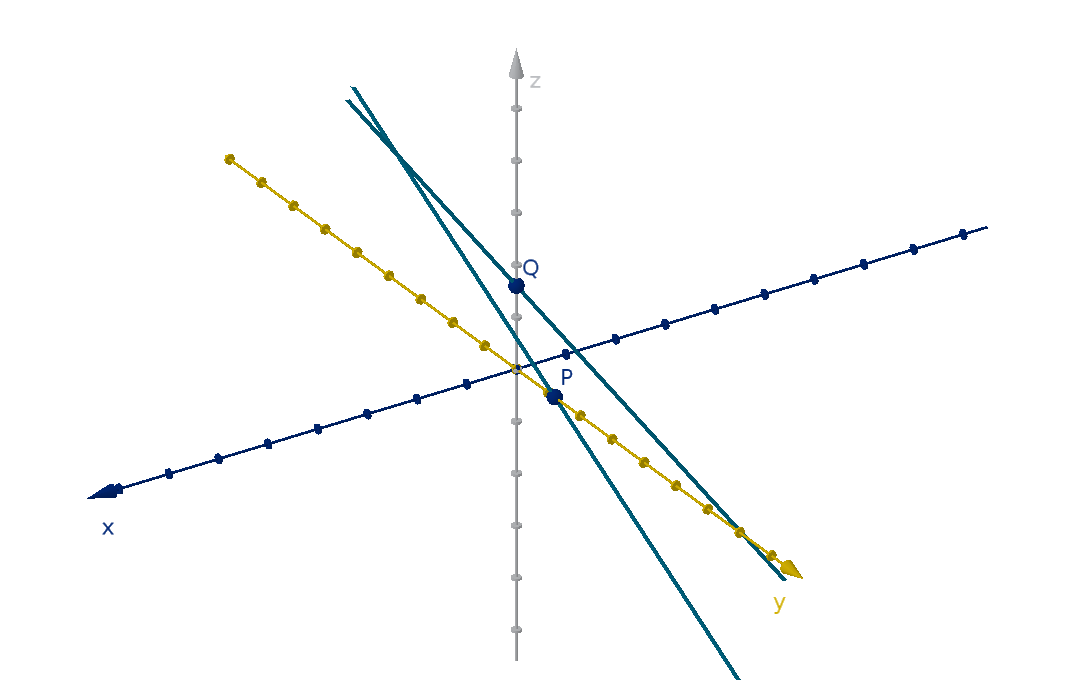
Figure: Two intersecting lines in three-space
97
Example 13.1.3
Other Plane Curves to Know
Graph the plane curves associated to the following vector functions:
a
r(t) = ⟨4 + 2t, 3 −3t⟩
b
r(t) = ⟨4 + 2t, 3 −3t⟩ 0 ≤ t ≤ 1
c
r(t) = ⟨3 cos t, 3 sin t⟩
d
r(t) =
t, t
3
98
Example 13.1.3
Other Plane Curves to Know
c
r(t) = ⟨3 cos t, 3 sin t⟩

99
Example 13.1.3
Other Plane Curves to Know
d
r(t) =
t, t
3

100
Example 13.1.3 Other Plane Curves to Know
Exercise
a Sketch the plane curve of
r(t) = (3 + t)
i + (5 −4t)
j 0 ≤ t ≤ 1.
b Sketch the plane curve of
r(t) = ⟨2 cos(t), 2 sin(t)⟩ 0 ≤ t ≤ 2π.
c How would
r(t) = ⟨2 cos(t), 2 sin(t) + 4⟩ 0 ≤ t ≤ 2π differ from
b ? Plot some points if you need to.
d How would
r(t) = ⟨6 cos(t), 2 sin(t)⟩ 0 ≤ t ≤ 2π differ from b ?
Does this plane curve have a shape you recognize?
e What graph is defined by
r(t) = (t
3
− 4t)
i + t
j?
101
Question 13.1.4
How Do We Visualize a Space Curve?
The space curve defined by
r(t) = (1 − cos(t) −sin(t))
i + cos(t)
j + sin(t)
k
is best understood as a projection.

Figure: A unit circle in the yx-plane projected onto x = 1 −y − z
102
Question 13.1.4
How Do We Visualize a Space Curve?
The space curve defined by
r(t) = t
i + t
2
j + t
3
k can be understood as
the intersection of two surfaces:

Figure: The intersection of z = x
3
and y = x
2
103
Question 13.1.4
How Do We Visualize a Space Curve?
The space curve defined by
r(t) = cos(t)
i + sin(t)
j +
t
4
k
can be understood by a projectile motion argument.

Figure:
r(t), which traces the unit circle above the xy-plane while steadily
increasing in the z-direction
104
Question 13.1.5
What Is the Limit of a Vector Function?
Definition
If
r(t) = ⟨f (t), g(t), h(t)⟩ then
lim
t→a
r(t) =
D
lim
t→a
f (t), lim
t→a
g(t), lim
t→a
h(t)
E
Provided the limits of all three component functions exist.
105
Question 13.1.5
What Is the Limit of a Vector Function?
Definition
A vector function
r is continuous at a if
lim
t→a
r(t) =
r(a).
This is the case if and only if the component functions f (t), g (t) and
h(t) are continuous at a.
106
Example 13.1.6
Testing Continuity
Is
r(t) = t
2
i + e
t
j +
sin t
t
k
continuous at t = 0? Justify your answer using the definition of
continuity.
107
Section 13.2
Derivatives of a Vector Functions
Goals:
1 Compute derivatives of vector functions.
2 Interpret derivatives as tangent vectors.
Question 13.2.1
What Is the Derivative of a Vector Function?
Definition
We define the derivative of
r(t) by
d
r
dt
=
r
′
(t) = lim
h→0
r(t + h) −
r(t)
h
Notice since the numerator is a vector and the denominator is a scalar,
we are taking the limit of a vector function.
109
Question 13.2.1
What Is the Derivative of a Vector Function?
If
r(t) = f (t)
i + g(t)
j then what is
r
′
(t)?
110
Question 13.2.1
What Is the Derivative of a Vector Function?
Theorem
If
r(t) = f (t)
i + g(t)
j then
r
′
(t) = f
′
(t)
i + g
′
(t)
j,
Provided these derivatives exist.
Similarly, if
r(t) = f (t)
i + g(t)
j + h(t)
k then
r
′
(t) = f
′
(t)
i + g
′
(t)
j + h
′
(t)
k,
Provided these derivatives exist.
111
Question 13.2.1
What Is the Derivative of a Vector Function?
The following properties follow from applying the derivative rules you
learned in single-variable calculus to each component of a vector function.
Theorem
For any differentiable vector functions
u(t),
v(t), differentiable
real-valued function f (t) and constant c we have
1 (
u +
v)
′
=
u
′
+
v
′
2 (c
u)
′
= c
u
′
3 (f
u)
′
= f
′
u + f
u
′
4 (
u ·
v)
′
=
u
′
·
v +
u ·
v
′
112
Question 13.2.2
What Is a Tangent Vector?
Definition
The vector
r
′
(t
0
) is called a tangent vector to the curve defined by
r(t).
If
r(t
0
) defines the point P, then we call
r
′
(t
0
) the tangent vector at P.
By replacing t
0
with a variable t, we can define the derivative function
r
′
(t).
113
Question 13.2.2
What Is a Tangent Vector?
If we imagine that
r(t) describes the position of an object at time t, then
r
′
(t) tells us the velocity (direction and magnitude) of the object.

Figure: A space curve and its tangent vector
114
Question 13.2.2
What Is a Tangent Vector?
Here are two closely related constructions to the tangent vector.
Definition
The unit tangent vector at
r(t
0
) is denoted
T (t
0
).
T (t
0
) =
r
′
(t
0
)
|
r
′
(t
0
)|
The tangent line to
r(t) at
r(t
0
) has the vector equation
L(s) =
r(t
0
) + s
r
′
(t
0
)
115
Section 14.1
Functions of Several Variables
Goals:
1 Convert an implicit function to an explicit function.
2 Calculate the domain of a multivariable function.
3 Calculate level curves and cross sections.
Question 14.1.1
What Is a Function of More than One Variable?
Definition
A function of two variables is a rule that assigns a number (the output)
to each ordered pair of real numbers (x, y) in its domain. The output is
denoted f (x, y).
Some functions can be defined algebraically. If
f (x, y) =
p
36 −4x
2
− y
2
then
f (1, 4) =
p
36 −4 · 1
2
− 4
2
= 4.
117
Example 14.1.2
The Domain of a Function
Identify the domain of f (x, y) =
p
36 −4x
2
− y
2
.
Figure: The domain of a function
118
Example 14.1.2
The Domain of a Function
Identify the domain of f (x, y) =
p
36 −4x
2
− y
2
.

Figure: The domain of a function
118
Application 14.1.3
Temperature Maps
Many useful functions cannot be defined algebraically. There is a
function T (x, y ) which gives the temperature at each latitude and
longitude (x, y) on earth.
T (−71.06, 42.36) = 50
T (−84.38, 33.75) = 59
T (−83.74, 42.28) = 41
Figure: A temperature map
119
Application 14.1.4
Digital Images
A digital image can be defined by a brightness function B(x, y).
y
x
687
1024
B(339, 773) = 158 B(340, 773) = 127
Figure: An image represented as a brightness function B on each pixel
120
Question 14.1.5
What Is the Graph of a Two-Variable Function?
Definition
The graph of a function f (x, y) is the set of all points (x, y, z) that
satisfy
z = f (x, y).
The height z above a point (x, y) represents the value of the function at
(x, y).
121
Question 14.1.5
What Is the Graph of a Two-Variable Function?
In this figure, f (1, 4) is equal to the height of the graph above (1, 4, 0).

Figure: The graph z =
p
36 −4x
2
− y
2
122
Question 14.1.6
How Do We Visualize a Graph in Three-Space?
Definition
A level set of a function f (x, y ) is the graph of the equation f (x, y) = c
for some constant c. For a function of two variables this graph lies in the
xy-plane and is called a level curve.
Example
Consider the function
f (x, y) =
p
36 −4x
2
− y
2
.
The level curve
p
36 −4x
2
− y
2
= 4 simplifies
to 4x
2
+ y
2
= 20. This is an ellipse.
Other level curves have the form
p
36 −4x
2
− y
2
= c or 4x
2
+ y
2
= 36 − c
2
.
These are larger or smaller ellipses.

123
Question 14.1.6
How Do We Visualize a Graph in Three-Space?
Level curves take their shape from the intersection of z = f (x, y) and
z = c. Seeing many level curves at once can help us visualize the shape
of the graph.

Figure: The graph z = f (x, y ), the planes z = c, and the level curves
124
Example 14.1.7
Drawing Level Curves
Where are the level curves on this temperature map?

Figure: A temperature map
125
Example 14.1.8
Using Level Curves to Describe a Graph
What features can we discern from the level curves of this topographical
map?
Figure: A topographical map
126
Example 14.1.9
A Cross Section
Definition
The intersection of a plane with a graph is a cross section. A level curve
is a type of cross section, but not all cross sections are level curves.
Find the cross section of z =
p
36 −4x
2
− y
2
at the plane y = 1.
127
Example 14.1.9
A Cross Section

Figure: The y = 1 cross section of z =
p
36 −4x
2
− y
2
128
Example 14.1.10
Converting an Implicit Equation to a Function
Definition
We sometimes call an equation in x, y and z an implicit equation.
Often in order to graph these, we convert them to explicit functions of
the form z = f (x, y)
Write the equation of a paraboloid x
2
− y + z
2
= 0 as one or more
explicit functions so it can be graphed. Then find the level curves.
129
Example 14.1.10
Converting an Implicit Equation to a Function

Figure: Level curves of x
2
− y + z
2
= 0
130
Question 14.1.11
How Does this Apply to Functions of More Variables?
We can define functions of three variables as well. Denoting them
f (x, y, z). For even more variables, we use x
1
through x
n
. The definitions
of this section can be extrapolated as follows.
Variables 2 3 n
Function f (x, y) f (x, y, z) f (x
1
, . . . , x
n
)
Domain subset of R
2
subset of R
3
subset of R
n
Graph z = f (x, y) in R
3
w = f (x, y, z) in R
4
x
n+1
= f (x
1
, . . . , x
n
) in R
n+1
Level Sets level curve in R
2
level surface in R
3
level set in R
n
131
Question 14.1.11
How Does this Apply to Functions of More Variables?
Observation
We might hope to solve an implicit equation of n variables to obtain an
explicit function of n −1 variables. However, we can also treat it as a
level set of an explicit function of n variables (whose graph lives in n + 1
dimensional space).
x
2
+ y
2
+ z
2
= 25
F (x, y , z) = x
2
+ y
2
+ z
2
F (x, y , z) = 25
f (x, y) = ±
p
25 −x
2
− y
2
Both viewpoints will be useful in the future.
132
Section 14.1
Summary Questions
Q1 What does the height of the graph z = f (x, y) represent?
Q2 What is the distinction between a level set and a cross section?
Q3 What are level sets in R
2
and R
3
called?
Q4 What is the difference between an implicit equation and explicit
function?
133
Section 14.1
Q50
Consider the implicit equation zx = y
a Rewrite this equation as an explicit function z = f (x, y).
b What is the domain of f ?
c Solve for and sketch a few level sets of f .
d What do the level sets tell you about the graph z = f (x, y)?
134
Section 14.1
Q50

134
Section 14.2
Limits and Continuity
Goals:
1 Understand the definition of a limit of a multivariable function.
2 Use the Squeeze Theorem
3 Apply the definition of continuity.
Question 14.2.1
What Is the Limit of a Function?
Definition
We write
lim
(x,y)→(a,b)
f (x, y) = L
if we can make the values of f stay arbitrarily close to L by restricting to
a sufficiently small neighborhood of (a, b).
Proving a limit exists requires a formula or rule. For any amount of
closeness required (ϵ), you must be able to produce a radius δ around
(a, b) sufficiently small to keep |f (x, y ) −L| < ϵ.
136
Example 14.2.2
A Limit That Does Not Exist
Show that lim
(x,y)→(0,0)
x
2
− y
2
x
2
+ y
2
does not exist.

137
Example 14.2.3
Another Limit That Does Not Exist
Show that lim
(x,y)→(0,0)
xy
x
2
+ y
2
does not exist.

138
Example 14.2.4
Yet Another Limit That Does Not Exist
Show that lim
(x,y)→(0,0)
xy
2
x
2
+ y
4
does not exist.

139
Question 14.2.5
What Tools Apply to Multi-Variable Limits?
The limit laws from single-variable limits transfer comfortably to
multi-variable functions.
1 Sum/Difference Rule
2 Constant Multiple Rule
3 Product/Quotient Rule
The Squeeze Theorem
If g < f < h in some neighborhood of (a, b) and
lim
(x,y)→(a,b)
g(x, y) = lim
(x,y)→(a,b)
h(x, y ) = L,
then
lim
(x,y)→(a,b)
f (x, y) = L.
140
Question 14.2.6
What Is a Continuous Function?
Definition
We say f (x, y) is continuous at (a, b) if
lim
(x,y)→(a,b)
f (x, y) = f (a, b).
Theorem
Polynomials, roots, trig functions, exponential functions and
logarithms are continuous on their domains.
Sums, differences, products, quotients and compositions of
continuous functions are continuous on their domains.
In each of our examples, the function was a quotient of polynomials, but
(0, 0) was not in the domain.
141
Question 14.2.6
What Is a Continuous Function?
Remark
Limits, continuity and these theorems can all be extrapolated to
functions of more variables.
142
Section 14.2
Summary Questions
Q1 Why is it harder to verify a limit of a multivariable function?
Q2 What do you need to check in order to determine whether a
function is continuous?
143
Section 14.3
Partial Derivatives
Goals:
1 Calculate partial derivatives.
2 Realize when not to calculate partial derivatives.
Question 14.3.1
What Is the Rate of Change of a Multivariable Function?
Motivational Example
The force due to gravity between two objects depends on their masses
and on the distance between them. Suppose at a distance of 8, 000km
the force between two particular objects is 100 newtons and at a distance
of 10, 000km, the force is 64 newtons.
How much do we expect the force between these objects to increase or
decrease per kilometer of distance?
145
Question 14.3.1
What Is the Rate of Change of a Multivariable Function?
Derivatives of a single-variable function were a way of measuring the
change in a function. Recall the following facts about f
′
(x).
1 Average rate of change is realized as the slope of a secant line:
f (x) − f (x
0
)
x − x
0
2 The derivative f
′
(x) is defined as a limit of slopes:
f
′
(x) = lim
h→0
f (x + h) − f (x)
h
3 The derivative is the instantaneous rate of change of f at x.
4 The derivative f
′
(x
0
) is realized geometrically as the slope of the
tangent line to y = f (x) at x
0
.
5 The equation of that tangent line can be written in point-slope form:
y − y
0
= f
′
(x
0
)(x − x
0
)
146
Question 14.3.1
What Is the Rate of Change of a Multivariable Function?
A partial derivative measures the rate of change of a multivariable
function as one variable changes, but the others remain constant.
Definition
The partial derivatives of a two-variable function f (x, y ) are the
functions
f
x
(x, y) = lim
h→0
f (x + h, y) −f (x, y )
h
and
f
y
(x, y) = lim
h→0
f (x, y + h) −f (x, y)
h
.
147
Question 14.3.1
What Is the Rate of Change of a Multivariable Function?
Notation
The partial derivative of a function can be denoted a variety of ways.
Here are some equivalent notations
f
x
∂f
∂x
∂z
∂x
∂
∂x
f
D
x
f
148
Example 14.3.2
Computing a Partial Derivative
Find
∂
∂y
(y
2
− x
2
+ 3x sin y ).
Main Idea
To compute a partial derivative f
y
, perform single-variable differentiation.
Treat y as the independent variable and x as a constant.
149
Synthesis 14.3.3
Interpreting Derivatives from Level Sets
Below are the level curves f (x, y) = c for some values of c. Can we tell
whether f
x
(−4, 1.25) and f
y
(−4, 1.25) are positive or negative?

Figure: Some level curves of f (x, y )
150
Question 14.3.4
What Is the Geometric Significance of a Partial Derivative?
The partial derivative f
x
(x
0
, y
0
) is realized geometrically as the slope of
the line tangent to z = f (x, y) at (x
0
, y
0
, z
0
) and traveling in the x
direction. Since y is held constant, this tangent line lives in y = y
0
.

Figure: The tangent line to z = f (x, y ) in the x direction
151
Example 14.3.5
Derivative Rules and Partial Derivatives
Find f
x
for the following functions f (x, y):
a f =
√
xy (on the domain x > 0, y > 0)
b f =
y
x
c f =
√
x + y
d f = sin (xy)
152
Question 14.3.6
What If We Have More than Two Variables?
We can also calculate partial derivatives of functions of more variables.
All variables but one are held to be constants. For example if
f (x, y, z) = x
2
− xy + cos(yz) −5z
3
then we can calculate
∂f
∂y
:
153
Example 14.3.7
A Function of Three Variables
For an ideal gas, we have the law P =
nRT
V
, where P is pressure, n is the
number of moles of gas molecules, T is the temperature, and V is the
volume.
a Calculate
∂P
∂V
.
b Calculate
∂P
∂T
.
c (Science Question) Suppose we’re heating a sealed gas contained in
a glass container. Does
∂P
∂T
tell us how quickly the pressure is
increasing per degree of temperature increase?
154
Question 14.3.8
How Do Higher Order Derivatives Work?
Taking a partial derivative of a partial derivative gives us a higher order
partial derivative. We use the following notation.
Notation
(f
x
)
x
= f
xx
=
∂
2
f
∂x
2
We need not use the same variable each time
Notation
(f
x
)
y
= f
xy
=
∂
∂y
∂
∂x
f =
∂
2
f
∂y∂x
155
Example 14.3.9
A Higher Order Partial Derivative
If f (x, y) = sin(3x + x
2
y) calculate f
xy
.
156
Question 14.3.10
Does Differentiation Order Matter?
No. Specifically, the following is due to Clairaut:
Theorem
If f is defined on a neighborhood of (a, b) and the functions f
xy
and f
yx
are both continuous on that neighborhood, then f
xy
(a, b) = f
yx
(a, b).
This readily generalizes to larger numbers of variables, and higher order
derivatives. For example f
xyyz
= f
zyxy
.
157
Section 14.3
Summary Questions
Q1 What is the role of each variable when we compute a partial
derivative?
Q2 What does the partial derivative f
y
(a, b) mean geometrically?
Q3 Can you think of an example where the partial derivative does not
accurately model the change in a function?
Q4 What is Clairaut’s Theorem?
158
Section 14.3
Q10
In the diagram from this example, use a point on the c = 30 level set to
approximate f
y
(4, −1.25).
Figure: Some level curves of f (x, y )
159
Section 14.3
Q20
Suppose Jinteki Corporation makes widgets which is sells for $100 each.
It commands a small enough portion of the market that its production
level does not affect the demand (price) for its products. If W is the
number of widgets produced and C is their operating cost, Jinteki’s
profit is modeled by
P = 100W − C .
Since
∂P
∂W
= 100 does this mean that increasing production can be
expected to increase profit at a rate of $100 per widget?
160
Section 14.3
Q28
How many third partial derivatives does a two-variable function have?
Assuming these derivatives are continuous, which of them are equal
according to Clairaut’s theorem?
161
Section 12.5
Normal Equations of Planes
Goals:
1 Give equations of planes in both vector and normal forms.
2 Use normal vectors to measure the distance to a plane.
Question 12.5.1
What Is the Slope-Intercept Equation of a Plane?
Unlike a line, a non-vertical plane has two slopes. One measures rise over
run in the x-direction, the other in the y -direction.

Figure: A plane with slopes in the x and y directions.
163
Question 12.5.1
What Is the Slope-Intercept Equation of a Plane?
Equation
A plane with z intercept (0, 0, b) and slopes m
x
and m
y
in the x and y
directions has equation
z = m
x
x + m
y
y + b.
164
Example 12.5.2
Writing the Equation of a Plane
Write the equation of a plane with intercepts (4, 0, 0), (0, 6, 0) and
(0, 0, 8).
165
Example 12.5.2
Writing the Equation of a Plane
Main Idea
Given three points in a plane A = (x
1
, y
1
, z
1
), B = (x
2
, y
2
, z
2
) and
C = (x
3
, y
3
, z
3
)
1 If two points share an x-coordinate, we can directly compute m
y
and vice versa.
2 Failing that, we can set up a system of equations and solve for m
x
,
m
y
and b.
166
Question 12.5.3
What is a Normal Vector to a Plane?
In algebra, you learned the normal equation of a line: e.g.
2x + 3y − 12 = 0. Why is it called this?

167
Question 12.5.3
What is a Normal Vector to a Plane?
In algebra, you learned the normal equation of a line: e.g.
2x + 3y − 12 = 0. Why is it called this?

167
Question 12.5.3
What is a Normal Vector to a Plane?
A normal vector to a plane is orthogonal to every vector in the plane.
Theorem
In three-dimensional space, every plane has normal vectors. They are all
parallel to each other.

Figure: A plane, its normal vector
n, and a vector
−→
PQ in the plane
168
Question 12.5.3
What is a Normal Vector to a Plane?
Theorem
If
r
0
= ⟨x
0
, y
0
, z
0
⟩ describes an known point on a plane, and
n = ⟨a, b, c⟩
is a normal vector. Then the normal equation of the plane is
(
r −
r
0
) ·
n = 0
or
a(x −x
0
) + b(y − y
0
) + c(z − z
0
) = 0
img/normalequation.png
Notice that since x
0
, y
0
and z
0
are constants, we can distribute and
collect them into a single term: d.
ax + by + cz − ax
0
− by
0
− cz
0
= 0
ax + by + cz + d = 0
169
Question 12.5.3
What is a Normal Vector to a Plane?
This reasoning works in any dimension to define a set of points whose
displacement from a known point is orthogonal to some normal vector.
Example
a(x −x
0
) + b(y − y
0
) = 0 defines a line.
a(x −x
0
) + b(y − y
0
) + c(z − z
0
) = 0 defines a plane.
a
1
(x
1
− c
1
) + a
2
(x
2
− c
2
) + ··· + a
n
(x
n
− c
n
) = 0 defines a
hyperplane.
170
Example 12.5.4
Computing a Normal Vector
Find the normal equation of the plane with intercepts (4, 0, 0), (0, 3, 0)
and (0, 0, 8). Compute a normal vector.
171
Synthesis 12.5.5
Using the Normal Vector to Compute Distance
Consider the line 2x + 3y − 12 = 0.
This is the line with normal vector
n = ⟨2, 3⟩ and known point P = (3, 2).
172
Synthesis 12.5.5
Using the Normal Vector to Compute Distance
Example
Let P
1
= (7, 2) and P
2
= (4, 0).
1 Draw the vectors
−−→
PP
1
and
−−→
PP
2
.
2 If you didn’t have a picture, how could you use the values of
n ·
−−→
PP
1
and
n ·
−−→
PP
2
to determine which side of the line P
1
and P
2
lie on?
173
Synthesis 12.5.5
Using the Normal Vector to Compute Distance
Theorem
Given a line, plane, or hyperplane with normal equation L(x
1
, . . . , x
k
) = 0
and corresponding normal vector
n, the signed distance from the
hyperplane to the point Q = (q
1
, . . . , q
k
) is
L(q
1
, . . . , q
k
)
|
n|
.
174
Example 12.5.6
The Distance from a Plane
Compute the geometric distance from the origin to the plane
6x + 8y + 3z − 24 = 0.
175
Application 12.5.7
Support Vector Machines
One type of machine learning involves training a computer to distinguish
between two states. For example, a computer might be trained to
distinguish between a cancerous tumor and a benign one.
To do this the computer is given a large set of cases. Each case is
measured by numerical data, such as:
The size of the tumor
The location of the tumor
The age of the patient
Results of blood tests
The brightness of each pixel in a CT scan or MRI
Each data type is a dimension, and each case is a point in a (probably
very high) dimensional space.
176
Application 12.5.7
Support Vector Machines

177
Section 12.5
Summary Questions
Q1 What information do you need in order to write the normal equation
of a plane?
Q2 How are the normal vectors of a plane related to each other?
Q3 What is the significance of the coefficients in the normal equation of
a plane?
Q4 How do we compute the signed distance from a point to a plane?
178
Section 12.5
Q14
Suppose we know the planes 12x + 18y + 6z − 15 = 0 and
ax + by + 4z + d = 0 are parallel. What can you say about the values of
a, b and d?
179
Section 12.5
Q30
Two planes are perpendicular if their normal vectors are orthogonal.
a Are 4x − 7y + z − 3 = 0 and 5x + y + 13z + 25 = 0 perpendicular?
b If two planes are perpendicular, is every vector in the first plane
orthogonal to every vector in the second plane?
180
Section 14.4
Linear Approximations
Goals:
1 Calculate the equation of a tangent plane.
2 Rewrite the tangent plane formula as a linearization or differential.
3 Use linearizations to estimate values of a function.
4 Use a differential to estimate the error in a calculation.
Question 14.4.1
What Is a Tangent Plane?
Definition
A tangent plane at a point P = (x
0
, y
0
, z
0
) on a surface is a plane
containing the tangent lines to the surface through P.

Figure: The tangent plane to z = f (x, y ) at a point
182
Question 14.4.1
What Is a Tangent Plane?
Equation
If the graph z = f (x, y) has a tangent plane at (x
0
, y
0
), then it has the
equation:
z − z
0
= f
x
(x
0
, y
0
)(x − x
0
) + f
y
(x
0
, y
0
)(y − y
0
).
Remarks
1 This is the point-slope form of the equation of a plane. f
x
(x
0
, y
0
)
and f
y
(x
0
, y
0
) are the slopes.
2 x
0
and y
0
are numbers, so f
x
(x
0
, y
0
) and f
y
(x
0
, y
0
) are numbers. The
variables in this equation are x, y and z.
183
Question 14.4.1
What Is a Tangent Plane?
The cross sections of the tangent plane give the equation of the tangent
lines we learned in single variable calculus.
y = y
0
x = x
0
z − z
0
= f
x
(x
0
, y
0
)(x − x
0
) + 0 z − z
0
= 0 + f
y
(x
0
, y
0
)(y − y
0
)


184
Example 14.4.2
Writing the Equation of a Tangent Plane
Give an equation of the tangent plane to f (x, y) =
√
xe
y
at (4, 0)
185
Question 14.4.3
How Do We Rewrite a Tangent Plane as a Function?
Definition
If we write z as a function L(x, y), we obtain the linearization of f at
(x
0
, y
0
).
L(x, y) = f (x
0
, y
0
) + f
x
(x
0
, y
0
)(x − x
0
) + f
y
(x
0
, y
0
)(y − y
0
)
If the graph z = f (x, y) has a tangent plane, then L(x, y) approximates
the values of f near (x
0
, y
0
).
Notice f (x
0
, y
0
) just calculates the value of z
0
. This formula is equivalent
to the tangent plane equation after we solve for z by adding z
0
to both
sides.
186
Example 14.4.4
Approximating a Function
Use a linearization to approximate the value of
√
4.02e
0.05
.
187
Question 14.4.5
How Does Differential Notation Work in More Variables?
The differential dz measures the change in the linearization of f (x, y)
given particular changes in the inputs: dx and dy. It is a useful
shorthand when one is estimating the error in an initial computation.
Definition
For z = f (x, y), the differential or total differential dz is a function of
a point (x
0
, y
0
) and two independent variables dx and dy.
dz = f
x
(x
0
, y
0
)dx + f
y
(x
0
, y
0
)dy
=
∂z
∂x
dx +
∂z
∂y
dy
Remark
The differential formula is just the tangent plane formula with
dz = z − z
0
dx = x −x
0
dy = y −y
0
.
188
Question 14.4.5
How Does Differential Notation Work in More Variables?
An old trigonometry application is to measure the height of a pole by
standing at some distance. We then measure the angle θ of incline to the
top, as well as the distance b to the base. The height is h = b tan θ.
a If the distance to the base is 13m and the angle of incline is
π
6
, what
is the height of the pole?
b Human measurement is never perfect. If our measurement of b is off
by at most 0.1m and our measurement of θ is off by at most
π
120
, use
a differential to approximate the maximum possible error in our h.
189
Section 14.4
Summary Questions
Q1 What do you need to compute in order to write the equation of a
tangent plane to z = f (x, y) at (x
0
, y
0
, z
0
)?
Q2 For what kinds of functions are linear approximations useful?
Q3 How are the tangent plane and the linearization related?
Q4 How is the differential defined for a two variable function? What
does each variable in the formula mean?
190
Section 14.4
Q10
Let g(x, y) =
3x
2
+4x−2
e
(y
3
)
. Write the equation of the tangent plane to
z = g(x, y) at (0, 1).
191
Section 14.4
Q16
Show how to use an appropriate linearization to approximate
1
5.12
sin
31π
30
.
a What function f (x, y) would you linearize to make this
approximation?
b What (x
0
, y
0
) would you use to write your linearization?
c What x and y would you plug into L(x, y) to approximate
1
5.12
sin
31π
30
?
192
Section 14.4
Q21
Boris is measuring the area of a rectangular field, so he can decide how
much grass seed to buy. According to his measurements, the field is 30m
by 50m, giving an area of 1500m
2
. If we accept that each of his
measurements has an error no larger than 0.2m, use a differential to
approximate the maximum error in his area computation.
193
Section 14.4
Q22
Suppose I decide to invest $10, 000 expecting a 6% annual rate of return
for 12 years, after which I’ll use it to purchase a house. The formula for
compound interest
P = P
0
e
rt
indicates that when I want to buy a house, I will have P = 10, 000e
0.72
.
I accept that my expected rate of return might have an error of up to
dr = 2%. Also, I may decide to buy a house up to dt = 3 years before or
after I expected.
a Write the formula for the differential dP at (r
0
, t
0
) = (0.06, 12).
b Given my assumptions, what is the maximum estimated error dP in
my initial calculation?
c What is the actual maximum error in P?
194
Section 14.4
Q24
Let f (x, y) be a function. What differential and what inputs into that
differential would you use to approximate f (5.5, 3.2) − f (4.7, 3.8).
195
Section 14.5
The Chain Rule
Goals:
1 Use the chain rule to compute derivatives of compositions of
functions.
2 Perform implicit differentiation using the chain rule.
Section 14.5 The Chain Rule
Motivational Example
Suppose Jinteki Corporation makes widgets which is sells for $100 each.
It commands a small enough portion of the market that its production
level does not affect the demand (price) for its products. If W is the
number of widgets produced and C is their operating cost, Jinteki’s
profit is modeled by
P = 100W − C
The partial derivative
∂P
∂W
= 100 does not correctly calculate the effect of
increasing production on profit. How can we calculate this correctly?
197
Question 14.5.1
How Do We Compute the Derivative of a Composition of Functions?
Given a function f (x, y) where x = x(t) and y = y(t), we can ask how f
changes as t changes. We can visualize this change by drawing the graph
z = f (x, y) over the path given by the parametric equations x(t) and
y(t).

Figure: The composition f (x(t), y(t)), represented by the height of z = f (x, y )
over the path (x (t), y (t))
198
Question 14.5.1
How Do We Compute the Derivative of a Composition of Functions?
Theorem (The Chain Rule)
Consider a differentiable function f (x, y). If we define x = x(t) and
y = y(t), both differential functions, we have
df
dt
=
∂f
∂x
dx
dt
+
∂f
∂y
dy
dt
199
Question 14.5.1
How Do We Compute the Derivative of a Composition of Functions?
Remarks
f (x(t), y(t)) is a function (only) of t. Because of this,
df
dt
is an
ordinary derivative, not a partial derivative.
df
dt
is not the slope of the composition graph.
slope =
rise in z
run in xy-plane
df
dt
=
rise in z
change in t
The chain rule is easy to remember because of its similarity to the
differential:
dz =
∂z
∂x
dx +
∂z
∂y
dy.
The proof is more complicated than just sticking a dt under each
term.
200
Example 14.5.2
Using the Chain Rule
If P = R − C and we have R = 100w and C = 3000 + 70w − 0.1w
2
,
calculate
dP
dw
.
201
Question 14.5.3
What If We Have More Variables?
The chain rule works just as well if x and y are functions of more than
one variable. In this case it computes partial derivatives.
Theorem
If f (x, y), x(s, t) and y(s, t), are all differentiable, then
∂f
∂s
=
∂f
∂x
∂x
∂s
+
∂f
∂y
∂y
∂s
202
Question 14.5.3
What If We Have More Variables?
We can also modify it for functions of more than two variables.
Theorem
Given f (x, y, z), x(t), y(t) and z(t), all differentiable, we have
df
dt
=
∂f
∂x
dx
dt
+
∂f
∂y
dy
dt
+
∂f
∂z
dz
dt
203
Example 14.5.4
A Composition with More Variables
Recall that for an ideal gas P(n, T , V ) =
nRT
V
. R is a constant. n is the
number of molecules of gas. T is the temperature in Celsius. V is the
volume in meters. Suppose we want to understand the rate at which the
pressure changes as an air-tight glass container of gas is heated.
a Apply the chain rule to get an expression for
dP
dT
.
b What is
dn
dT
?
c What is
dT
dT
?
d Suppose that
dV
dT
= (5.9 × 10
−6
)V . Calculate and simplify the
expression you got for
dP
dT
.
204
Example 14.5.4
A Composition with More Variables
Recall that for an ideal gas P(n, T , V ) =
nRT
V
. R is a constant. n is the
number of molecules of gas. T is the temperature in Celsius. V is the
volume in meters. Suppose we want to understand the rate at which the
pressure changes as an air-tight glass container of gas is heated.
a Apply the chain rule to get an expression for
dP
dT
.
204
Example 14.5.4
A Composition with More Variables
Recall that for an ideal gas P(n, T , V ) =
nRT
V
. R is a constant. n is the
number of molecules of gas. T is the temperature in Celsius. V is the
volume in meters. Suppose we want to understand the rate at which the
pressure changes as an air-tight glass container of gas is heated.
b What is
dn
dT
?
204
Example 14.5.4
A Composition with More Variables
Recall that for an ideal gas P(n, T , V ) =
nRT
V
. R is a constant. n is the
number of molecules of gas. T is the temperature in Celsius. V is the
volume in meters. Suppose we want to understand the rate at which the
pressure changes as an air-tight glass container of gas is heated.
c What is
dT
dT
?
204
Example 14.5.4
A Composition with More Variables
Recall that for an ideal gas P(n, T , V ) =
nRT
V
. R is a constant. n is the
number of molecules of gas. T is the temperature in Celsius. V is the
volume in meters. Suppose we want to understand the rate at which the
pressure changes as an air-tight glass container of gas is heated.
d Suppose that
dV
dT
= (5.9 × 10
−6
)V . Calculate and simplify the
expression you got for
dP
dT
.
204
Example 14.5.5
A Composition with Limited Information
Suppose g(p, q, r) = re
p
2
q
. Given that p, q, r are all differentiable
functions of x with the values in the following table, compute
dg
dx
when
x = 2.
x 0 1 2 3
p(x) 3 1 5 10
p
′
(x) −3 2 3 4
q(x) 6 2 −2 3
q
′
(x) −1 −5 2 3
r(x) 10 11 7 3
r
′
(x) 1 0 −1 −3
205
Application 14.5.6
Implicit Differentiation
Recall that an implicit equation on n variables defines a level set of a
n-variable function. Consider the graph x
3
+ y
2
− 4xy = 0. How can we
use this to calculate
dy
dx
at the point (3, 3)?
206
Application 14.5.6
Implicit Differentiation
Figure: The graph of F (x, y ) = x
3
+ y
2
− 4xy = 0, its tangent line at (3, 3),
and the gradient of F
Main Ideas
dy
dx
is the slope of the tangent line to F (x, y ) = c.
The chain rule allows us to derive
dy
dx
= −
F
x
F
y
−
F
x
F
y
is the negative reciprocal of
F
y
F
x
, which is the slope of ∇F .
207
Application 14.5.7
Indirect Profit Functions
Suppose a firm chooses how much quantity q to produce, but their profit
Π(q, α) depends on some parameter α outside their control (maybe a tax
or a measure of regulatory burden). The firm, once it knows the value of
α, will choose the q that maximizes profit. How will their profit change
as α changes?
208
Application 14.5.7
Indirect Profit Functions
Figure: Two graphs of z = Π(q, α), one where q changes to be the optimal
choice for each α and one where q is fixed at q
0
, the optimal choice for α
0
209
Section 14.5
Summary Questions
Q1 How can we visualize f (x, y), when x and y are functions of t?
Q2 Explain why
df
dt
cannot be interpreted as a slope of f over the
xy-plane.
Q3 What is the difference between
dz
dx
and
∂z
∂x
? How is the first one
computed?
Q4 How do you use the chain rule to differentiate implicit functions?
210
Section 14.5
Q12
Liam says “Suppose f is a function of x and y. If x and y are increasing,
then f is increasing.” We all know Liam is incorrect. How could we use
the chain rule to refute him?
211
Section 14.5
Q14
Let x = t
2
and y = sin t. Let f (x, y) = xy.
a Compute
df
dt
using the multivariable chain rule.
b Compute
df
dt
by substituting and using single-variable differentiation.
c What earlier rule of differentiation can we recover by applying the
chain rule to f (x, y) = xy?
212
Section 14.5
Q26
Another principle in physics is the conservation of energy. Kenetic energy
is given by E =
1
2
mv
2
, where m is the mass and v is the linear speed of
the object. Suppose that we have a rock drifiting through space.
Suppose it impacts stationary rocks and the combined mass sticks
together (without releasing any energy as heat, light or sound). Thus the
mass of the total travelling object increases, while the total energy stays
the same. Derive an expression for how speed changes per unit of
increase in mass.
213
Section 14.5
Q27
Suppose that x is a function of t and that when t = 9, we have x = 7
and
dx
dt
= −3. Define f (x, t) =
√
x + t.
a Compute the partial derivate
∂f
∂t
(7, 9).
b Compute the total derivative
df
dt
(7, 9).
c In a few sentences, explain what these two quantities compute and
why they are different from each other.
214
Section 14.5
Q30
Suppose the position of a particle at time t is given by
x(t) = t
2
y(t) = 3 − t
z(t) =
√
t
At t = 4, how quickly is particle travelling away from the plane
x + 2y − 2z = 10?
215
Section 14.5
Q31
Here is a diagram of the level curves of h(x, y ) for certain values of c.
a Is h
y
(2, 1) positive or negative? Explain in a sentence or two.
b Add a vector to the diagram that indicates the direction of greatest
increase of h at (−2, 0).
c Suppose x = 4 −5t and y = 3t
2
. Determine, with the aid of a
relevant calculation, whether
dh
dt
is positive or negative at t = 1.
216
Section 14.6
The Gradient Vector
Goals:
1 Calculate the gradient vector of a function.
2 Relate the gradient vector to the shape of a graph and its level
curves.
3 Compute directional derivatives.
Question 14.6.1
How Do We Compute Rates of Change in Another Direction?
The partial derivatives of f (x, y) give the instantaneous rate of change in
the x and y directions. This is realized geometrically as the slope of the
tangent line. What if we want to travel in a different direction?
Figure: The tangent line to z = f (x, y ) in the x direction
218
Question 14.6.1
How Do We Compute Rates of Change in Another Direction?
Definition
Let f (x, y) be a function and
u be a unit vector in R
2
. The directional
derivative, denoted D
u
f , is the instantaneous rate of change of f as we
move in the
u direction. This is also the slope of the tangent line to
z = f (x, y) in the direction of
u.

Figure: The tangent line to f (x, y ) in the direction of
u
219
Question 14.6.1
How Do We Compute Rates of Change in Another Direction?
Recall that we compute D
x
f by comparing the values of f at (x, y) to
the value at (x + h, y), a displacement of h in the x-direction.
D
x
f (x, y) = lim
h→0
f (x + h, y) −f (x, y )
h
To compute D
u
f for
u = a
i + b
j, we compare the value of f at (x, y ) to
the value at (x + ta, y + tb), a displacement of t in the
u-direction.
Limit Formula
D
u
f (x, y) = lim
t→0
f (x + ta, y + tb) −f (x, y )
t
220
Question 14.6.1
How Do We Compute Rates of Change in Another Direction?
Questions:
1 What direction produces the greatest directional derivative? The
smallest?
2 How are these directions related to the geometry (specifically the
level curves) of the graph?
3 How these directions related to the partial derivatives?
221
Question 14.6.1
How Do We Compute Rates of Change in Another Direction?

Figure: A cross section of z = f (x, y ) and a tangent line in the direction of
u
222
Question 14.6.2
What Is the Gradient Vector?
Definition
The gradient vector of f at (x, y) is
∇f (x, y) = ⟨f
x
(x, y), f
y
(x, y)⟩
Remarks:
1 The gradient vector is a function of (x, y). Different points have
different gradients.
2
u
max
, which maximizes D
u
f , points in the same direction as ∇f .
3
u
0
, which is tangent to the level curves, is orthogonal to ∇f .
223
Question 14.6.3
How Do We Compute a Directional Derivative?
The tangent lines live in the tangent plane. We can compute their slope
by rise over run.
Let
u be a unit vector from (x
0
, y
0
) to (x
1
, y
1
). Let the associated z
values in the tangent plane be z
0
and z
1
respectively.
D
u
f (x
0
, y
0
) =
rise
run
=
z
1
− z
0
|
u|
=f
x
(x
0
, y
0
)(x
1
− x
0
) + f
y
(x
0
, y
0
)(y
1
− y
0
)
=∇f (x
0
, y
0
) ·
u.

224
Question 14.6.3
How Do We Compute a Directional Derivative?
Functions of More Variables
We can also define directional derivatives of higher variable functions
with analogous results.
f (x
1
, . . . , x
n
) is a differentiable function.
u is a unit vector in R
n
.
D
u
f denotes the directional derivative in the direction of
u.
∇f = ⟨f
x
1
, . . . , f
x
n
⟩ is an n-dimensional vector function on R
n
.
D
u
f = ∇f ·
u
225
Synthesis 14.6.4
Directional Derivative and the Cosine Formula
Now that we have a formula for directional derivatives, we can verify our
observations from earlier. Suppose f (x, y ) is a differentiable function and
we can choose any unit vector
u.
a Write D
u
f (x, y) in terms of the length of a vector and an angle.
b In what direction
u will f increase fastest?
c What will be the value of D
u
f (x, y) in that direction?
d In what direction
u will D
u
f (x, y) = 0?
226
Synthesis 14.6.4
Directional Derivative and the Cosine Formula
Figure: The angle between the gradient of f and a unit vector
Main Ideas
The cosine formula for the dot product lets us relate the directional
derivative to an angle.
f increases fastest in the direction of ∇f (x, y).
D
u
f (x, y) = 0 when ∇f (x, y) and
u are orthogonal.
227
Example 14.6.5
A Directional Derivative
Let f (x, y) =
p
9 −x
2
− y
2
and let
u = ⟨0.6, −0.8⟩.
a What are the level curves of f ?
b What direction does ∇f (1, 2) point?
c Without calculating, is D
u
f (1, 2) positive or negative?
d Calculate ∇f (1, 2) and D
u
f (1, 2).
228
Example 14.6.6
Drawing the Gradient
Let h(x, y ) give the altitude at longitude x and latitude y . Assuming h is
differentiable, draw the direction of ∇h(x, y ) at each of the points
labeled below. Which gradient is the longest?
A
B
C
Figure: A topographical map
229
Application 14.6.7
Edge Detection
The length of the gradient of a brightness function detects the edges in a
picture, where the brightness is changing quickly.
∂B
∂x
(336, 785) ≈
185−187
1
∂B
∂y
(336, 785) ≈
179−187
1
∇B(336, 785) ≈ (−2, −8)
∂B
∂x
(340, 784) ≈
97−139
1
∂B
∂y
(340, 784) ≈
72−139
1
∇B(340, 784) ≈ (−42, −67)
∇B
∇B
Figure: A long gradient vector indicates a swift change in brightness. Its
direction suggests the shape of the edges.
230
Application 14.6.8
Tangent Planes to a Level Surface
Use a gradient vector to find the equation of the tangent plane to the
graph x
2
+ y
2
+ z
2
= 14 at the point (2, 1, −3).
231
Application 14.6.8
Tangent Planes to a Level Surface
Main Idea
The graph of an implicit equation can be written as a level set of a
function. The gradient of that function is a normal vector to the level set
and also to its tangent line/plane/hyperplane.

Figure: The level surface x
2
+ y
2
+ z
2
= 14, its tangent plane and ∇F .
232
Section 14.6
Summary Questions
Q1 What does the direction of the gradient vector tell you?
Q2 What does the directional derivative mean geometrically?
Q3 How do you compute a directional derivative?
Q4 How is the gradient vector related to a level set?
233
Section 14.6
Q12
Suppose the linearization of f (x, y) at (−3, 9) has the equation
L(x, y) = 4 + 2(x + 3) −
1
3
(y − 9).
What is the slope of L from (−3, 9) to (5, 3)?
234
Section 14.6
Q14
If D
u
f (x, y) < 0, what can you say about the directions of ∇f (x, y) and
u?
235
Section 14.6
Q16
Explain why it makes sense that if D
u
f (a, b, c) = 0, then
u is tangent to
the level surface of f through (a, b, c).
236
Section 14.6
Q26
The brightness function on the Mona Lisa image ranges from 0 to 255. If
we use adjacent points to apporixmate the gradient as in the example,
what is the longest gradient vector we could theoretically produce?
237
Section 14.6
Q28
Let P be a point on the circle x
2
+ y
2
= r
2
. Show that the position
vector of P is normal to the circle at P.
238
Section 14.6
Q36
Suppose that f (x, y, z) is a differentiable function, and f (3, 5, −2) = 13.
Suppose further that the vectors ⟨3, 1, 0⟩ and ⟨0, 2, 5⟩ both lie in the
tangent plane to the surface f (x, y, z) = 13 at (3, 5, −2). If the
maximum value of D
u
f (3, 5, −2) is 20, find all possible values of
∇f (3, 5, −2).
239
Section 14.7
Maximum and Minimum Values
Goals:
1 Find critical points of a function.
2 Test critical points to find local maximums and minimums.
3 Use the Extreme Value Theorem to find the global maximum and
global minimum of a function over a closed set.
Question 14.7.1
What Are Local Extremes?
The local extremes of a function are the local minimums and
maximums.
Definition
Given an n-variable function f (x
1
, x
2
, . . . , x
n
) we say that a point P in
n-space is
1 a local maximum if f (P) ≥ f (Q) for all Q in some neighborhood
around P.
2 a local minimum if f (P) ≤ f (Q) for all Q in some neighborhood
around P.
241
Question 14.7.2
Where Do Local Extremes Lie?
In the case of a two-variable function, we can visualize this as follows: If
f
x
(P) = 0, then we could travel in the x direction to increase or decrease
f . If f
y
(P) = 0, then we could travel in the y direction to increase or
decrease f . Thus at a local maximum or local minimum, the tangent
plane must be horizontal.

Figure: Tangent lines must have slope 0 at a local max.
242
Question 14.7.2
Where Do Local Extremes Lie?
Definition
We say P is a critical point of f if either
1 ∇f (P) =
0 or
2 ∇f (P) does not exist (because one of the partial derivatives does
not exist).
Theorem
The local maximums and minimums of a function can only occur at
critical points.
243
Example 14.7.3
Finding Critical Points
The function z = 2x
2
+ 4x + y
2
−6y + 13 has a minimum value. Find it.
244
Question 14.7.4
How Do We Identify Two-Variable Local Maximums and Minimums?
A critical point could be a local maximum. In this case f curves
downward in every direction.

Figure: A local maximum at (0, 0)
245
Question 14.7.4
How Do We Identify Two-Variable Local Maximums and Minimums?
A critical point could be a local minimum. In this case f curves upward
in every direction.

Figure: A local minimum at (0, 0)
246
Question 14.7.4
How Do We Identify Two-Variable Local Maximums and Minimums?
A critical point could be neither. f curves upward in some directions but
downward in others. This configuration is called a saddle point.

Figure: A saddle point at (0, 0)
247
Question 14.7.4
How Do We Identify Two-Variable Local Maximums and Minimums?
Theorem (The Second Derivatives Test)
Suppose f is differentiable at (P) and f
x
(P) = f
y
(P) = 0. Then we can
compute
D = f
xx
(P)f
yy
(P) − [f
xy
(P)]
2
1 If D > 0 and f
xx
(P) > 0 then P is a local minimum.
2 If D > 0 and f
xx
(P) < 0 then P is a local maximum.
3 If D < 0 then P is a saddle point.
Unfortunately, if D = 0, this test gives no information.
248
Question 14.7.4
How Do We Identify Two-Variable Local Maximums and Minimums?
Definition
The quantity D in the second derivatives test is actually the determinant
of a matrix called the Hessian of f .
f
xx
(P)f
yy
(P) − [f
xy
(P)]
2
= det
f
xx
(P) f
xy
(P)
f
yx
(P) f
yy
(P)
| {z }
Hf (P)
Hf follows a logical pattern and can be a useful mnemonic for the second
derivatives test.
249
Example 14.7.5
Classifying a Critical Point
Let f (x, y) = cos(2x + y) + xy
a Verify that ∇f (0, 0) = ⟨0, 0⟩.
b Is (0, 0) a local minimum, a local maximum, or neither?
250
Example 14.7.5
Classifying a Critical Point

Figure: The graph z = cos(2x + y) + xy with a local maximum at (0, 0)
251
Question 14.7.6
How Do We Find Global Extremes?
Theorem (The Extreme Value Theorem)
A continuous function f on a closed and bounded domain D has a global
maximum and a global minimum somewhere in D.
Definition
Let D be a subset of n-space.
D is closed if it contains all of the points on its boundary.
D is bounded if there is some upper limit to how far its points get
from the origin (or any other fixed point). If there are points of D
arbitrarily far from the origin, then D is unbounded.
252
Question 14.7.6
How Do We Find Global Extremes?
For one-variable functions. The EVT requires that the domain be a union
of finite, closed intervals (and maybe finitely many isolated points).

Figure: A union of finite, closed intervals
253
Question 14.7.6
How Do We Find Global Extremes?

Figure: x
2
+ y
2
≤ 9 is closed.

Figure: x
2
+ y
2
< 9 is not
closed.
254
Question 14.7.6
How Do We Find Global Extremes?

Figure: −2 ≤ x ≤ 2 and
−3 < y < 3 is not closed.

Figure: −2 ≤ x ≤ 2 and
−3 ≤ y ≤ 3 and (x, y ) = (1, 2)
is not closed.
255
Question 14.7.6
How Do We Find Global Extremes?

Figure: −2 ≤ x ≤ 2 and
−3 ≤ y ≤ 3 is bounded.

Figure: −2 ≤ x ≤ 2 is
unbounded.
256
Example 14.7.7
Finding a Global Maximum
Consider the function f (x, y) = x
2
+ 2y
2
− x
2
y on the domain
D = {(x, y) : x
2
+ y
2
≤ 16, x ≤ 0}
a Does f have a maximum value on D? How do we know?
b Find the critical points of f .
c Must one of the critical points be the maximum?
d Find the maximum of f .
257
Example 14.7.7
Finding a Global Maximum
Consider the function f (x, y) = x
2
+ 2y
2
− x
2
y on the domain
D = { (x, y)
|{z}
points in R
2
: x
2
+ y
2
≤ 16, x ≤ 0
| {z }
conditions
}
a Does f have a maximum value on D? How do we know?
257
Example 14.7.7
Finding a Global Maximum
Consider the function f (x, y) = x
2
+ 2y
2
− x
2
y on the domain
D = { (x, y)
|{z}
points in R
2
: x
2
+ y
2
≤ 16, x ≤ 0
| {z }
conditions
}
a Does f have a maximum value on D? How do we know?
257
Example 14.7.7
Finding a Global Maximum
Consider the function f (x, y) = x
2
+ 2y
2
− x
2
y on the domain
D = { (x, y)
|{z}
points in R
2
: x
2
+ y
2
≤ 16, x ≤ 0
| {z }
conditions
}
a Find the critical points of f .
257
Example 14.7.7
Finding a Global Maximum
Consider the function f (x, y) = x
2
+ 2y
2
− x
2
y on the domain
D = { (x, y)
|{z}
points in R
2
: x
2
+ y
2
≤ 16, x ≤ 0
| {z }
conditions
}
a Must one of the critical points be the maximum?
257
Example 14.7.7
Finding a Global Maximum
Consider the function f (x, y) = x
2
+ 2y
2
− x
2
y on the domain
D = { (x, y)
|{z}
points in R
2
: x
2
+ y
2
≤ 16, x ≤ 0
| {z }
conditions
}
a Find the maximum of f .
257
Example 14.7.7
Finding a Global Maximum

257
Example 14.7.7
Finding a Global Maximum
Main Ideas
If the Extreme Value Theorem applies, then all we need to do is find
the critical points and evaluate f at each. One is guaranteed to be
the maximum, and one is guaranteed to be the minimum.
∇f =
0 will detect critical points on the interior, but not on the
boundary.
We can rewrite the function on a boundary component using
substitution. Set the derivative equal to 0 to find critical points.
Derivatives will not detect maximums at the endpoints of a boundary
curve. These must be included in your set of critical points.
258
Section 14.7
Summary Questions
Q1 Where must the local maximums and minimums of a function
occur? Why does this make sense?
Q2 What does the second derivatives test tell us?
Q3 What hypotheses does the Extreme Value Theorem require? What
does it tell us?
Q4 Assuming a maximum and minimum exist, where must you look in a
domain to be sure you find them?
259
Section 14.7
Q6
Is a global maximum also a local maximum? Explain.
260
Section 14.7
Q12
Suppose f (x) is a function of x with critical points x = a and x = b.
Suppose g(y) is a function of y with critical points y = c and y = d.
What are the critical points of h(x, y ) = f (x) + g(y )?
261
Section 14.7
Q16
For what values of a does f (x, y) = x
2
+ y
2
+ axy have a local minimum
at the origin?
262
Section 14.7
Q32
Let f (x, y) be a differentiable function and let
D = {(x, y) : y ≥ x
2
− 4, x ≥ 0, y ≤ 5}.
a Sketch the domain D.
b Does the Extreme Value Theorem guarantee that f has an absolute
minimum on D? Explain.
c List all the places you would need to check in order to locate the
minimum.
263
Section 14.8
Lagrange Multipliers
Goals:
1 Find minimum and maximum values of a function subject to a
constraint.
2 If necessary, use Lagrange multipliers.
Question 14.8.1
What Is a Constraint?
Sometimes we aren’t interested in the maximum value of f (x, y ) over the
whole domain, we want to restrict to only those points that satisfy a
certain constraint equation.
The maximum on the constraint
is unlikely to be the same as the
unconstrained maximum (where
∇f = 0). Can we still use ∇f
to find the maximum on the
constraint?

Figure: Maximizing f such that
x + y = 1
265
Question 14.8.2
How Do We Solve a Constrained Optimization?
The method of Lagrange Multipliers makes use of the following
theorem.
Theorem
Suppose an objective function f (x, y ) and a constraint function
g(x, y) are differentiable. The local extremes of f (x, y ) given the
constraint g(x, y) = c occur where
∇f = λ∇g
for some number λ, or else where ∇g = 0. The number λ is called a
Lagrange Multiplier.
This theorem generalizes to functions of more variables.
266
Question 14.8.2
How Do We Solve a Constrained Optimization?

Figure: Where ∇f is not parallel to ∇g , we can travel along g (x, y ) = c and
increase the value of f . This is because D
u
f > 0 for some
u along the
constraint.
267
Example 14.8.3
The Maximum on a Curve
Find the point(s) on the ellipse 4x
2
+ y
2
= 4 on which the function
f (x, y) = xy is maximized.
268
Example 14.8.3
The Maximum on a Curve

Figure: The four points that satisfy ∇f = λ∇g and g(x, y) = c.
Main Idea
The level set of a continuous (constraint) function is always closed. If it
is also bounded and the objective function is differentiable, then one of
the points produced by Lagrange multipliers will be the global maximum
and one will be the global minimum of the constrained optimization.
269
Example 14.8.4
The Maximum on a Surface
Find the maximum value of the function f (x, y, z) = x
4
y
4
z on the
sphere x
2
+ y
2
+ z
2
= 36.

Figure: The gradient vector and level surface of a constraint function and the
gradient vector of the objective function
270
Synthesis 14.8.5
Using the Extreme Value Theorem and Lagrange Multipliers
How can Lagrange multipliers help us find the maximum of
f (x, y) = x
2
+ 2y
2
− x
2
y on the domain
D = {(x, y) : x
2
+ y
2
≤ 16, x ≤ 0}?
271
Synthesis 14.8.5
Using the Extreme Value Theorem and Lagrange Multipliers
Main Idea
To find the absolute minimum and maximum of a differentiable function
f (x, y) over a closed and bounded domain D:
1 Compute ∇f and find the critical points inside D.
2 Identify the boundary components. Find the critical points on each
using substitution or Lagrange multipliers.
3 Identify the endpoints (intersections) of the boundary components.
4 Evaluate f (x, y) at all of the above. The minimum is the lowest
number, the maximum is the highest.
272
Question 14.8.7
Can This Lagrange Apply to More Than One Constraint?
If we have two constraints in three-space, g(x, y, z) = c and
h(x, y , z) = d, then their intersection is generally a curve.

Figure: The intersection of the constraints g (x, y, z) = c and h(x, y , z) = d
273
Question 14.8.7
Can This Lagrange Apply to More Than One Constraint?
According to our earlier argument about directional derivatives, at a
maximum P on the constraint, ∇f (P) must be normal to the constraint.
There are more ways for this to happen with two constraint equations.
1 ∇f (P) could be parallel to ∇g (P).
2 ∇f (P) could be parallel to ∇h(P).
3 ∇f (P) could be the vector sum of a vector parallel to ∇g (P) and a
vector parallel to ∇h(P).
274
Question 14.8.7
Can This Lagrange Apply to More Than One Constraint?
Theorem
If f (x, y, z) is a differentiable function and g (x, y , z) = c and
h(x, y , z) = d are two constraints. If P is a maximum of f (x, y , z)
among the points that satisfy these constraints then either
∇f (P) = λ∇g (P) + µ∇h(P)
for some scalars λ and µ, or ∇g(P) and ∇h(P) are parallel.
This system of equations is usually difficult to solve by hand.
275
Question 14.8.7
Can This Lagrange Apply to More Than One Constraint?
Remark
You can check the reasonableness of this method by noting that it gives
us a system of 5 variables, x, y , z, λ, µ, and five equations:
f
x
(x, y, z) = λg
x
(x, y, z) + µh
x
(x, y, z) g(x, y, z) = c
f
y
(x, y, z) = λg
y
(x, y, z) + µh
y
(x, y, z) h(x, y , z) = d
f
z
(x, y, z) = λg
z
(x, y, z) + µh
z
(x, y, z)
We therefore generally expect this system to have a finite number of
solutions, though there are plenty of counterexamples to this expectation.
276
Section 14.8
Summary Questions
Q1 What is a constraint?
Q2 What equations do you write when you apply the method of
Lagrange multipliers?
Q3 Is the set of points that satisfies a constraint closed and bounded?
Explain.
Q4 How does a constraint arise when finding the maximum over a
closed and bounded domain?
277
Section 14.8
Q8
Suppose the curve below is the graph of g(x, y) = k. Use methods from
calculus to find and mark the approximate location of the point that
maximizes the function f (x, y) = 3y −x subject to the constraint
g(x, y) = k. Justify your reasoning in a few sentences.
278
Section 14.8
Q10
Show that (3, 3) is not a local maximum of
f (x, y) = 2x
2
− 4xy + y
2
− 8x on the graph x
3
+ y
3
= 6xy .
279
Section 14.8
Q18
Consider the following two questions:
Find the maximum value of f (x, y) that satisfies x
2
+ y
2
≤ 9.
Find the maximum value of f (x, y) that satisfies x
2
+ y
2
= 9.
a How are the questions different?
b Which question takes less work to solve? Explain how you know.
c Do solutions exist to both questions? What additional information
would guarantee that they do?
280
Section 14.8
Q20
Consider the function f (x, y) = x
2
+ 6xy + 9y
2
+ 5. Find the maximum
and minimum values of f on the domain
D = {(x, y) : y ≥ x, x ≥ 0, x
2
+ y
2
≤ 10}
281
Section 15.1
Double Integrals
Goals:
1 Approximate the volume under a graph by adding prisms.
2 Calculate the volume under a graph using a double integral.
Question 15.1.1
How Do We Approximate the Volume Under z = f (x, y )?
We approximated the area under the graph y = f (x) by rectangles.
Smaller rectangles give a better approximation, and we defined the limit
of these approximations to be the definite integral.
Z
b
a
f (x)dx = lim
∆x→0
n
X
i=1
f (x
∗
i
)∆x
Figure: The area under y = f (x) approximated by rectangles
283
Question 15.1.1
How Do We Approximate the Volume Under z = f (x, y )?
A similar method approximates the signed volume under the graph
z = f (x, y) (where volume below the xy-plane counts as negative). We
divide the domain

0 ≤ x ≤ 4
0 ≤ y ≤ 2
into subrectangles of area A. We
draw a prism over each rectangle
whose height is the value of the
function over some test point
(x
∗
i
, y
∗
i
).
Volume ≈
n
X
i=1
f (x
∗
i
, y
∗
i
)A.
284
Question 15.1.1
How Do We Approximate the Volume Under z = f (x, y )?
If our domain is not a rectangle, we may not be able to divide it into
subrectangles. Luckily, the formula for volume of a prism works for any
shape base. We can still compute
Volume ≈
n
X
i=1
f (x
∗
i
, y
∗
i
)A
i
.

Figure: A domain subdivided into irregular subregions
285
Question 15.1.1
How Do We Approximate the Volume Under z = f (x, y )?
For a reasonably well-behaved function f (x, y), the actual volume can be
computed by taking a limit of these approximations. We call this limit
the double-integral.
Definition
Let D be a domain in R
2
. For a given division of D into n subregions
denote
A
i
, the area of the i
th
region.
(x
∗
i
, y
∗
i
), any point in the i
th
region
|A| is the diameter of the largest region.
We define the double integral of f (x, y) to be a limit over all possible
divisions of D.
ZZ
D
f (x, y)dA = lim
|A|→0
n
X
i=1
f (x
∗
i
, y
∗
i
)A
i
286
Example 15.1.2
Approximating a Double Integral
Consider
ZZ
D
x
2
ydA, where D is the region shown here. Approximate
the integral using the division of D shown, and evaluating f (x, y ) at the
midpoint of each rectangle.
x
y
1
21
287
Question 15.1.3
How Do We Evaluate Double Integrals?
We already know another way of computing a volume. We can compute
the area of the cross sections perpendicular to the x-axis. Let the
function A(x) denote this area at each x. Then
Volume =
Z
b
a
A(x) dx
A(x) is itself the area under a curve. In a particular cross section, x is
constant, and f (x, y) is a function of y . The area below this graph is the
integral
A(x) =
Z
d
c
f (x, y) dy
We can put these together to obtain an iterated integral, an integral
whose integrand is itself an integral.
288
Question 15.1.3
How Do We Evaluate Double Integrals?

Figure: Cross sections of the region below the graph: z = f (x, y )
289
Question 15.1.3
How Do We Evaluate Double Integrals?
Theorem (Fubini’s Theorem)
For any domain D we have
ZZ
D
f (x, y) dA =
Z
b
a
Z
d
c
f (x, y) dy
dx
where a and b are the x bounds of D, and c and d are the y bounds of
the cross section at each x. Alternately, we can write
ZZ
D
f (x, y) dA =
Z
d
c
Z
b
a
f (x, y) dx
dy
where c and d are the y bounds of D, and a and b are the x bounds of
the cross section at each y.
290
Example 15.1.4
Using Fubini’s Theorem
Compute
ZZ
D
x
2
y dA, where D is the region shown here:
x
y
1
21
291
Question 15.1.5
Can We Break a Double Integral into a Product of Single Integrals?
In general, we can’t expect to factor out the inner integral of
RR
D
f (x, y)dydx (using the constant multiple rule). The y-bounds may
depend on x, and the y terms may not factor out of the integrand.
However, for certain functions and domains, this factoring is possible.
Theorem
Z
b
a
Z
d
c
f (x)g (y )dydx =
Z
b
a
f (x)dx
Z
d
c
g(y)dy
We won’t be able to use this theorem all the time. It has two important
requirements:
1 The bounds of integration (a, b, c, d) are constants. We’ll see
integrals soon where this is not the case.
2 The integrand can be factored into a function of x times a function
of y. Most two-variable functions cannot.
292
Example 15.1.6
Integrating a Product
Use a product decomposition to compute
RR
D
x
2
ydA, where D is the
region shown here:
x
y
1
21
293
Application 15.1.7
Rates (per Area)
Single integrals can compute total change given a rate of change.
meters traveled per second −→ total meters traveled.
GDP growth per year −→ total GDP growth.
mass of a chemical produced per second −→ total mass produced.
294
Application 15.1.7
Rates (per Area)
Integrating rainfall per square kilometer gives the total rain that fell in a
watershed.

Figure: A rainfall density map
295
Application 15.1.7
Rates (per Area)
Integrating watts per square meter on a solar array gives the total energy
generated.

Figure: Solar panels
By Jud McCranie - Own work, CC BY-SA 4.0
https://commons.wikimedia.org/w/index.php?curid=70132767
296
Application 15.1.8
Probability
If we generate a data set in which we have measured two variables, then
the probability that a random data point lies in a given region is the
double integral of a joint density function over that area.

Figure: A highly correlated set of observations and an uncorrelated joint density
function
297
Section 15.1
Summary Questions
Q1 What shape do we use to approximate volume under a surface?
Q2 What formula do we use to compute the exact volume under a
graph z = f (x, y)?
Q3 What does Fubini’s Theorem tell us?
Q4 What conditions do you need in order to write a double integral as a
product of single integrals?
298
Section 15.1
Q10
Let T be the triangle with vertices (0, 0), (1, 0) and (0, 2). Show how to
approximate
ZZ
T
e
x+y
dA by dividing T into four right triangles with
legs of length 1 and
1
2
. Use the midpoint of the hypotenuses as the test
points.
299
Section 15.1
Q12
Let R be the rectangle
R = {(x, y) : − 2 ≤ x ≤ 2, −1 ≤ y ≤ 1}.
Let S be the solid region above R and below the graph z = x
2
y + xy
2
.
Write a function A(x) which gives the area of the cross section of S
perpendicular to the x-axis at each value of x.
300
Section 15.2
Double Integrals over General Regions
Goals:
1 Set up double integrals over regions that are not rectangles.
2 Evaluate integrals where the bounds contain variables.
3 Decide when to make
R
dy the outer integral, and compute the
change of bounds.
Example 15.2.1
Integrating Over a Polygon
Let D be the triangle with vertices (0, 0), (4, 0) and (4, 2). Calculate
ZZ
D
4xy dA
302
Example 15.2.1
Integrating Over a Polygon
Let D be the triangle with vertices (0, 0), (4, 0) and (4, 2). Calculate
ZZ
D
4xy dA

302
Example 15.2.1
Integrating Over a Polygon
Main Idea
To find the bounds of a double integral
1 Find the x value where the domain begins and ends. These numbers
are the bounds of the outer integral.
2 Find the functions (of the form y = g(x)) which define the top and
bottom of the domain. These functions are the bounds of the inner
integral.
303
Question 15.2.2
What Are the Integral Laws for Double Integrals?
Some single variable integral laws apply to double integrals as well
(provided the integrals exist).
1 The sum rule:
ZZ
D
f (x, y) + g (x, y)dA =
ZZ
D
f (x, y)dA +
ZZ
D
g(x, y)dA
2 The constant multiple rule:
ZZ
D
cf (x, y)dA = c
ZZ
D
f (x, y)dA
3 If D is the union of two non-overlapping subdomains D
1
and D
2
then
ZZ
D
f (x, y)dA =
ZZ
D
1
f (x, y)dA +
ZZ
D
2
f (x, y)dA
304
Example 15.2.3
A Region Without a (Single) Bottom Curve
Let D be the region bounded by y =
√
x, y = 0 and y = x −6. Calculate
ZZ
D
(x + y) dA.
305
Example 15.2.3
A Region Without a (Single) Bottom Curve
Let D be the region bounded by y =
√
x, y = 0 and y = x −6. Calculate
ZZ
D
(x + y) dA.

305
Example 15.2.4
Using Anti-Symmetry
Let D be the region x
2
+ y
2
≤ 9. Evaluate
ZZ
D
3
√
x
p
y + 3dA.
306
Example 15.2.4
Using Anti-Symmetry
Let D be the region x
2
+ y
2
≤ 9. Evaluate
ZZ
D
3
√
x
p
y + 3dA.

306
Example 15.2.4
Using Anti-Symmetry
Main Idea
We can argue that an integral
ZZ
D
f (x, y)dA is equal to zero when
1 D is symmetric about some line L. If we folded it over L, one side
of D would lie exactly on the other side.
2 f is antisymmetric about L. For each point (x, y ) in D the image
of (x, y) across L, denoted r
L
(x, y) has the property:
f (r
L
(x, y)) = −f (x, y).

307
Example 15.2.5
Using Order to Manipulate the Integrand
Let D be the triangle with vertices (0, 0),
(0, 2) and (1, 2). Calculate
ZZ
D
e
(y
2
)
dA.

308
Example 15.2.5
Using Order to Manipulate the Integrand
Main Idea
If we don’t know the anti-derivative of an integrand with respect to one
variable, try switching the order of integration.
Remember to change the bounds too.
309
Application 15.2.6
Area of a Domain
Theorem
The area of a region D can be calculated:
ZZ
D
1 dA.
310
Application 15.2.6
Area of a Domain

Figure: A solid of height 1 over a domain D
311
Section 15.4
Applications of Double Integrals
Goals:
1 Integrate a probability distribution to calculate a probability.
Application 15.4.1
Using Integrals to Compute Probabilities
Most probabilities that people think about are discreet.
A flipped coin has a
1
2
chance to be heads,
1
2
to be tails.
A random M&M has a
1
6
chance to be red,
1
6
orange,
1
6
yellow,
1
6
green,
1
6
blue and
1
6
brown.
313
Application 15.4.1
Using Integrals to Compute Probabilities
On the other hand, a person’s chance of being exactly 68 inches tall is
zero. Even people who say they are 5
′
8
′′
are slightly more or slightly less.
Instead we can ask what your chance is of being between 68 and 69
inches tall.
Definition
A function f is a probability density function for an event, if the
chance of an outcome between a and b is
R
b
a
f (x)dx.

314
Application 15.4.1
Using Integrals to Compute Probabilities
Definition
A function f is a joint probability density function for a pair random
events if the chance that the outcome (x, y) lies in D is
ZZ
D
f (x, y) dA.
315
Application 15.4.1 Using Integrals to Compute Probabilities
Exercise
Darmok and Jalad each travel to the island of Tanagra and arrive
between noon and 4PM. Let (x, y ) represent their respective arrival times
in hours after noon. Suppose the probability that (x, y ) falls in a certain
domain D which is a subset of {(x, y ) : 0 ≤ x ≤ 4, 0 ≤ y ≤ 4} is
RR
D
x
32
dydx.
Calculate the probability that:
1 Darmok arrives after 3PM.
2 Jalad arrives before 1PM.
3 They both arrive before 2PM.
4 Darmok arrives before Jalad.
5 They arrive within an hour of each other (set it up, don’t evaluate).
6 What does the distribution say about when Darmok is likely to
arrive? What about Jalad?
316
Section 15.2
Summary Questions
Q1 What are the steps for writing a double integral over a general
region?
Q2 How do you decide whether dx or dy is the inner variable?
Q3 What is antisymmetry, and how can we use it to evaluate integrals?
Q4 How can we use a double integral to compute the area of a region?
317
Section 15.2
Q8
Let D be the parallelogram with vertices (0, 1), (0, 4), (5, 3) and (5, 6).
Let f (x, y) be a continuous function.
a Set up the bounds of integration of
ZZ
D
f (x, y) dA.
b Could we save time by computing
Z
5
0
Z
4
1
f (x, y) dydx instead?
Explain.
318
Section 15.2
Q18
Consider the integral
Z
6
−6
Z
0
−
√
36−y
2
x
2
dxdy. Write this integral in the
order dydx.
319
Section 15.2
Q20
Let g(x, y) = x
3
e
y
2
. Argue that
Z
4
−4
Z
3
−3
g(x, y) dydx = 0.
320
Section 15.2
Q24
Suppose you are given that f (x, y) = −f (−y, −x). Over what domains
D can we argue by symmetry that
ZZ
D
f (x, y) dA = 0? Draw an
example of one.
321
Section 15.2
Q32
Consider the integral
Z
4
−4
Z
6
0
x
3
√
ydydx
a Show how to approximate the value of this integral, dividing the
domain into sub-rectangles of length 2 units and width 3 units and
using the lower right corners as test points. You should evaluate any
functions that appear in your estimate, but you do not need to
simplify the arithmetic.
b Explain in a sentence or two how you can determine the exact value
of this integral without calculating any anti-derivatives.
c Discuss what test point you could have picked in a , such that your
approximation would have computed the exact value of the integral.
Note: There are several relevant observations to make in response to
this question.
322
Section 15.6
Triple Integrals
Goals:
1 Set up triple integrals over three-dimensional domains.
2 Evaluate triple integrals.
Question 15.6.1
How Do We Integrate a Three-Variable Function?
Definition
Given a domain D in three dimension space, and a function f (x, y, z).
We can subdivide D into regions
V
i
is the volume of the i
th
region.
(x
∗
i
, y
∗
i
, z
∗
i
) is a point in the i
th
region.
V is the diameter of the largest region.
We define the triple integral of f over D to be the following limit over
all possible divisions of D:
ZZZ
D
f (x, y, z) dV = lim
V →0
n
X
i=1
f (x
∗
i
, y
∗
i
, z
∗
i
)V
i
324
Question 15.6.1
How Do We Integrate a Three-Variable Function?
Fubini’s theorem applies to triple integrals as well. We write them as
iterated integrals.
Theorem
ZZZ
D
f (x, y, z)dV =
Z
x
2
x
1
Z
y
2
y
1
Z
z
2
z
1
f (x, y, z) dzdydx
where
z
1
and z
2
are the bounds of z, which may be functions of x and y.
y
1
and y
2
are the bounds of y, which may be functions of x.
x
1
and x
2
are the bounds of x. They are numbers.
The variables of can also be reordered, with the bounds defined
analogously.
325
Example 15.6.2
Integrating Over a Prism
Let R = {(x, y, z) : 0 ≤ x ≤ 4, 0 ≤ y ≤ 2, 0 ≤ z ≤ 3}. Compute
ZZZ
R
3zy + x
2
dV .
326
Example 15.6.2
Integrating Over a Prism
Let R = {(x, y, z) : 0 ≤ x ≤ 4, 0 ≤ y ≤ 2, 0 ≤ z ≤ 3}. Compute
ZZZ
R
3zy + x
2
dV .

Figure: A Rectangular Prism
326
Question 15.6.3
How Do We Interpret Triple Integrals Geometrically?
Z
3
0
f (x, y, z) dz computes the area under the graph w = f (x, y , z) over
each vertical segment of the form (x, y) = (x
0
, y
0
) in the domain. It is a
function of x and y.

Figure:
Z
3
0
f (x, y , z) dz, represented as an area in a zw-plane
327
Question 15.6.3
How Do We Interpret Triple Integrals Geometrically?
Z
2
0
Z
3
0
f (x, y, z) dzdy computes the volume under the graph
w = f (x, y, z) over each x = x
0
cross-section of the domain. It is a
function of x.

Figure:
Z
2
0
Z
3
0
f (x, y , z) dzdy , represented as a volume in yzw -space
328
Application 15.6.4
Triple Integrals in Math and Science
1 Integrating a function ρ(x, y , z), which gives the density of an object
at each point, gives the total mass of the object.
2 Integrating xρ(x, y , z), yρ(x, y , z) and zρ(x, y , z) gives the center
of mass of the object.
3 Integrating a three-dimensional probability distribution over a region
gives the probability that the triple (X , Y , Z ) lies in that region.
4 Integrating 1 dV over a region gives the volume of that region.
329
Application 15.6.4
Triple Integrals in Math and Science
Density lets us visualize a triple integral without referring to a fourth
(geometric) dimension.
Z
3
0
f (x, y, z) dz computes
the density of the vertical
segments at each (x, y).
Z
2
0
Z
3
0
f (x, y, z) dzdy
computes the density of the
rectangle at each x.

Z
4
0
Z
2
0
Z
3
0
f (x, y, z) dzdydx computes the total mass of the prism.
330
Example 15.6.5
Integrating Over an Irregular Region
Let R be the region above the xy plane, below the cylinder x
2
+ z
2
= 16
and between y = 0 and y = 3. Compute
ZZZ
R
4yz dV .
331
Example 15.6.5
Integrating Over an Irregular Region
Let R be the region above the xy plane, below the cylinder x
2
+ z
2
= 16
and between y = 0 and y = 3. Compute
ZZZ
R
4yz dV .

Figure: The region between x
2
+ y
2
= 16 and the xy-plane
331
Example 15.6.5
Integrating Over an Irregular Region
Main Idea
The following approach will produce the bounds of a region with a top
surface and a bottom surface.
1 The z bounds are given by the equations z = f (x, y) and
z = g(x, y) of the top and bottom surface.
2 The intersection of the top and bottom surface can produce relevant
bounds on x and y. We can graph these, along with any given
bounds involving x and y.
3 After drawing the bounded region in the xy-plane, the x and y
bounds are computed as for a double integral.
Like with double integrals, we will want to break the region into smaller
pieces in some cases. In other cases, we may want to change the order of
integration.
332
Example 15.6.6
A Solid Given by Vertices
Suppose we want to integrate over T , the tetrahedron (pyramid) with
vertices (0, 0, 0), (4, 0, 0), (4, 2, 0) and (4, 0, 2). How would we set up the
bounds of integration?
333
Example 15.6.6
A Solid Given by Vertices

Figure: z bounds of T

Figure: x, y bounds of T
334
Example 15.6.7
Changing the Order of Integration
Suppose D is the bounded region enclosed between the graph of
y = 4x
2
+ z
2
and the plane y = 4. Set up the bounds of the integral
ZZZ
D
f (x, y, z)dV .
Figure: A region bounded by a paraboloid and a plane
335
Example 15.6.7
Changing the Order of Integration
Suppose D is the bounded region enclosed between the graph of
y = 4x
2
+ z
2
and the plane y = 4. Set up the bounds of the integral
ZZZ
D
f (x, y, z)dV .

Figure: A region bounded by a paraboloid and a plane
335
Question 15.6.8
When Does a Triple Integral Decompose as a Product?
The product theorem from double integrals also works here:
Theorem
If y
1
, y
2
, z
1
and z
2
are constants, then
Z
x
2
x
1
Z
y
2
y
1
Z
z
2
z
1
f (x)g (y )h(z) dzdydx
=
Z
x
2
x
1
f (x) dx
Z
y
2
y
1
g(y) dy
Z
z
2
z
1
h(z) dz
336
Question 15.6.8
When Does a Triple Integral Decompose as a Product?
Example
Along with the sum and constant multiple rules we can simplify
Z
4
0
Z
2
0
Z
3
0
3zy + x
2
dzdydx
to obtain the following:
Z
4
0
Z
2
0
Z
3
0
3zy dzdydx +
Z
4
0
Z
2
0
Z
3
0
x
2
dzdydx
=3
Z
4
0
dx
Z
2
0
y dy
Z
3
0
z dz +
Z
4
0
x
2
dx
Z
2
0
dy
Z
3
0
dz
=3 ·4
Z
2
0
y dy
Z
3
0
z dz + 2 ·3
Z
4
0
x
2
dx
337
Section 15.6
Summary Questions
Q1 What does Fubini’s theorem say about integrals with dV ?
Q2 How is density used to understand triple integrals. Why wasn’t it
necessary or appropriate for double integrals?
Q3 How do you find the bounds of the inner variable in a triple integral?
Q4 How to you find the bounds of the other two variables?
338
Section 15.6
Q26
Let R be the region enclosed by y =
√
25 −x
2
, z = 6 −y and z =
√
y.
Set up the bounds of
RRR
R
g(x, y, z)dV .
339
Section 15.6
Q26

Figure: The region enclosed by x
2
+ y
2
= 25, z = 6 − y , and z =
√
y
340
Section 15.6
Q20
Cheng is integrating over R, the region given by x
2
+ y
2
+ z
2
≤ 25. He
gives the following setup. Is this valid?
Z
√
25−y
2
−z
2
−
√
25−y
2
−z
2
Z
√
25−x
2
−z
2
−
√
25−x
2
−z
2
Z
√
25−x
2
−y
2
−
√
25−x
2
−y
2
f (x, y, z) dzdydx
341
Section 15.6
Q20

341
Section 15.6
Q22
Let R = {(x, y, z) : z ≤ 2x − y , z ≥ 0, y ≥ x
2
}. Compute
ZZZ
R
xz dV .
342
Section 15.6
Q36
Rewrite the integral
Z
2
0
Z
2
2−x
Z
4−x
2
0
f (x, y, z) dzdydx as an integral with
the differential dxdzdy.
343
Section 15.6
Q36

344
Section 15.6
Q38
Let S = {(x, y, z) : x
2
+ y
2
+ z
2
≤ 25}. Explain why
ZZZ
S
x
3
y
4
cos πz dV cannot be decomposed as a product.
345
Section 15.9
Change of Variables in Multiple Integrals
Goals:
1 Calculate a Jacobian
2 Convert a multivariable integral from one coordinate system to
another.
Question 15.9.1
How Does u -Substitution Work?
In a u-substitution, we do not just change the variable and the bounds.
We also need to account for width changing from ∆x to ∆u.
Figure:
Z
π/2
0
2 sin(2x) dx =
Z
π
0
2 sin(u) du.
Instead we need to divide to account for the extra width of each
rectangle.
347
Question 15.9.1
How Does u-Substitution Work?
We cannot always just divide by a constant. The ratio of widths may be
different at different values of x and u.
Figure:
Z
√
π
0
2 sin(x
2
) dx =
Z
π
0
2 sin(u) du.
The way we solve this is with a differential. We write du =
du
dx
dx.
348
Question 15.9.1
How Does u-Substitution Work?
The rule du =
du
dx
dx can actually be used to our advantage.
Example
If u = x
2
, then du = 2x dx. We can use this to perform a substitution
like:
Z
√
π
0
2x sin(x
2
) dx =
Z
π
0
sin(u) du
Note we have to change three things
1 The integrand: sin(x
2
) → sin(u)
2 The bounds: 0 → 0 and
√
π → π
3 The differential: 2x dx → du
Remark
In single-variable calculus we use substitution to handle integrals with
difficult integrands. In multivariable calculus, we will mostly use
substitution to handle integrals with difficult domains.
349
Question 15.9.2
How Does a Two-Variable Substitution Work?
To perform a two-variable substitution, it is helpful to have the following
formula for computing area.
Formula
Given vectors
a = ⟨a
x
, a
y
⟩ and
b = ⟨b
x
, b
y
⟩, the parallelogram formed by
a and
b has
Area =
det
a
x
a
y
b
x
b
y
= |a
x
b
y
− b
x
a
y
|
350
Question 15.9.2
How Does a Two-Variable Substitution Work?
Main Idea
In the case of a linear substitution like
r(u, v ) = ⟨a
x
u + b
x
v, a
y
u + b
y
v⟩
a unit uv square maps to a parallelogram with sides ⟨a
x
, a
y
⟩ and ⟨b
x
, b
y
⟩
in the xy-plane. We can fix the area distortion produced by substituting
x and y for u and v by setting
dxdy = |a
x
b
y
− b
x
a
y
|dudv.
Question
How can we handle non-linear substitutions?
351
Example 15.9.3
Parabolic Coordinates
Our main source of substitutions are alternative coordinate systems for
the plane. Here is some parabolic graph paper. Each point has
coordinates (σ, τ). The gold curves are σ = 0, 1, 2, 3, . . .. The blue
curves are τ = 0, 1, 2, 3, . . ..

352
Example 15.9.3
Parabolic Coordinates
Formula
For a given point (σ, τ), we can calculate the corresponding (x, y )
coordinates:
x = στ
y =
1
2
(τ
2
− σ
2
)
We can express this as a function
r(σ, τ ) =
στ,
1
2
(τ
2
− σ
2
)
.
353
Example 15.9.3
Parabolic Coordinates
Suppose we want to integrate the function f (x, y) = x
2
over the domain
below left. It’s easier to describe this domain in (σ, τ) coordinates.
1 The bounds of integration are 2 ≤ σ ≤ 5, and 3 ≤ τ ≤ 5.
2 We can substitute the integrand: x
2
= σ
2
τ
2
.
3 But
Z
5
2
Z
5
3
σ
2
τ
2
dτ dσ computes the volume over the rectangle
(below right), not over our domain, which provides a larger base.


354
Example 15.9.3
Parabolic Coordinates
When we take a dσ by dτ rectangle in a Cartesian coordinate system,
how much bigger does it get when we map it into the parabolic
coordinate system? It is too difficult to compute it precisely. Instead, we
can approximate the effect of dσ and dτ by differentials.
∂
r
∂σ
=
∂x
∂σ
,
∂y
∂σ
∂
r
∂τ
=
∂x
∂τ
,
∂y
∂τ
355
Example 15.9.3
Parabolic Coordinates
We now have the final ingredient to rewrite
RR
D
x
2
dA where D is the
domain below.
356
Question 15.9.4
How Does a Two-Variable Substitution Work Generally?
Definition
Given a two-variable vector function
r(u, v ) = ⟨x(u, v ), y(u, v )⟩,
J =
∂x
∂u
∂y
∂u
∂x
∂v
∂y
∂v
is called the Jacobian matrix. The Jacobian is the absolute value of
the determinant and is denoted:
∂(x, y )
∂(u , v)
= |det J|
=
∂x
∂u
∂y
∂v
−
∂y
∂u
∂x
∂v
We will define the Jacobian similarly for a three variable vector function.
357
Question 15.9.4
How Does a Two-Variable Substitution Work Generally?
Main Idea
When performing two-variable integration, if we want to substitute u and
v for x and y, then our differential is replaced as follows:
dxdy =
∂(x, y )
∂(u , v)
dudv
=
∂x
∂u
∂y
∂v
−
∂y
∂u
∂x
∂v
dudv
Remark
Parabolic coordinates are not very useful. The kinds of regions they
describe nicely almost never appear naturally. They are a used here only
to demonstrate the theory of multivariable substitution.
358
Section 15.3
Double Integrals in Polar Coordinates
Goals:
1 Convert integrals from Cartesian to polar coordinates.
2 Evaluate integrals in polar coordinates.
Question 15.3.1
What Are Polar Coordinates?
Definition
The polar coordinates of a point are denoted (r, θ) where
θ (“theta”) is the direction to the point from the origin (measured
anticlockwise from the positive x axis).
r is the distance to the point in that direction (negative r means
travel backwards).
Unlike Cartesian coordinates, a point can be represented in several
different ways.
(1, 0) = (1, 2π) = (1, 4π).
(1, 0) = (−1, π)
(0, α) = (0, β) for all α, β.
360
Question 15.3.1 What Are Polar Coordinates?
Exercise
Plot and label the following points and sets in polar coordinates
A = (2,
π
3
)
B = (1.5, 3π)
C = (−3, −
π
4
)
R = {(r, θ) : 0 ≤ r ≤ 2}
S = {(r , θ) :
π
6
≤ θ ≤
π
4
, r ≥ 1}
361
Question 15.3.1 What Are Polar Coordinates?
Cartesian to Polar
p(r , θ) = r cos(θ)
i + r sin(θ)
j
x = r cos θ
y = r sin θ
Notice: x
2
+ y
2
= r
2
r =
p
x
2
+ y
2
θ =
(
tan
−1
y
x
x > 0
tan
−1
y
x
+ π x < 0
A full circle is 0 ≤ θ ≤ 2π.
362
Question 15.3.2
What Is the Jacobian of Polar Coordinates?
Calculate the Jacobian
∂(x, y )
∂(r, θ)
such that dxdy =
∂(x, y )
∂(r, θ)
drdθ.
363
Question 15.3.2
What Is the Jacobian of Polar Coordinates?
Main Idea
The Jacobian of polar coordinates is r. Thus
dydx = rdrdθ
364
Example 15.3.3
Integrating Over a Disc
Let D be the disk: x
2
+ y
2
≤ 9. Calculate
ZZ
D
p
x
2
+ y
2
dA.
365
Example 15.3.3
Integrating Over a Disc
Let D be the disk: x
2
+ y
2
≤ 9. Calculate
ZZ
D
p
x
2
+ y
2
dA.
365
Example 15.3.4
Integrating Over a Wedge
Let D = {(x, y) : x ≥ 0, x ≤ y, x
2
+ y
2
≤ 2}. Sketch D and calculate
ZZ
D
x
2
dA.
366
Example 15.3.4
../imgicons/teacher.pdf
Integrating Over a Wedge
Trig Formulas
Higher powers of sine and cosine arise naturally in polar integrals. You’ll
be responsible for applying the following formulas.
Formulas
sin
2
θ =
1
2
−
cos(2θ)
2
cos
2
θ =
1
2
+
cos(2θ)
2
sin
3
θ = sin θ − cos
2
θ sin θ
cos
3
θ = cos θ − sin
2
θ cos θ
367
Example 15.3.4 Integrating Over a Wedge
Exercise
For each of the integrals below, sketch the domain of integration then
convert to polar. You need not evaluate.
1
ZZ
D
2x − 3y
2
dydx
where D = {(x, y) : x
2
+ y
2
≤ 16, −y ≤ x ≤ y }
2
ZZ
D
x
2
ydydx
where D = {(x, y) : 4 ≤ x
2
+ y
2
≤ 9, y ≤ 0}
3
Z
3
−3
Z
√
9−y
2
0
x
2
+ y
2
dxdy
Which of your integrals can be solved using the product formula?
368
Example 15.3.5
A Circle Through the Origin
Let D be the domain (x − 1)
2
+ y
2
≤ 1. Evaluate
ZZ
D
x
2
+ y
2
dA.
369
Example 15.3.6
Polar Coordinates in Triple Integrals
Set up the integral for f (x, y, z) over the region R enclosed between the
graphs z = x
2
+ y
2
and z =
p
6 −x
2
− y
2
.
370
Example 15.3.6
Polar Coordinates in Triple Integrals
Set up the integral for f (x, y, z) over the region R enclosed between the
graphs z = x
2
+ y
2
and z =
p
6 −x
2
− y
2
.
370
Example 15.3.6
Polar Coordinates in Triple Integrals
Main Idea
When setting up a triple integral, sometimes the domain of the outer two
variables (usually x and y) is more conveniently written in polar
coordinates.
Remark
The coordinate system (r, θ, z) is called the cylindrical coordinate
system.
371
Section 15.8
Triple Integrals in Spherical Coordinates
Goals:
1 Write integrals in spherical coordinates
Question 15.8.1
What Are Spherical Coordinates?
Spherical coordinates are a three dimensional coordinate system. Here ρ
(“rho”) is the (three dimensional) distance from the origin. ϕ (“phi”) is
the angle the segment from the origin makes with the positive z axis. θ
is the angle that the projection to the xy-plane makes with the positive
x-axis.
373
Question 15.8.1
What Are Spherical Coordinates?
The following formulas follow from trigonometry.
Cartesian to Spherical
x = ρ cos θ sin ϕ
y = ρ sin θ sin ϕ
z = ρ cos ϕ
Notice: x
2
+ y
2
+ z
2
= ρ
2
A full sphere is 0 ≤ θ ≤ 2π
0 ≤ ϕ ≤ π
374
Question 15.8.1 What Are Spherical Coordinates?
Exercise
Describe (or draw?) the following regions in spherical coordinates.
1 R = {(ρ, θ, ϕ) : ϕ =
π
2
}
2 R = {(ρ, θ, ϕ) : ρ ≤ 5}
3 R = {(ρ, θ, ϕ) : 0 ≤ θ ≤
π
4
}
4 R = {(ρ, θ, ϕ) : ϕ ≥
2π
3
}
375
Question 15.8.1 What Are Spherical Coordinates?
Theorem
The Jacobian for spherical coordinates is
ρ
2
sin ϕ.
376
Example 15.8.2
The Volume of a Sphere
Calculate the volume of a sphere of radius R.
377
Example 15.8.3
Converting to Spherical Coordinates
Convert the following triple integral to spherical coordinates:
Z
3
0
Z
0
−
√
9−x
2
Z
√
9−x
2
−y
2
0
yz
2
dzdydx
378
Example 15.8.3
Converting to Spherical Coordinates
Convert the following triple integral to spherical coordinates:
Z
3
0
Z
0
−
√
9−x
2
Z
√
9−x
2
−y
2
0
yz
2
dzdydx
378
Question 15.8.4
When Do We Use Spherical Coordinates?
Spherical coordinates are only worth using if the domain is reasonably
well behaved.
1 In many cases, all the bounds of integration are constants.
2 The bounds of ρ involve the expression x
2
+ y
2
+ z
2
.
3 The bounds of θ are given by inequalities containing only x and y.
Draw these in the plane.
4 The bounds of ϕ are given by inequalities concerning z.
5 In some more advanced applications, the ρ bounds may be a
function of ϕ or θ, meaning ρ should be the inner variable.
379
Question 15.8.4 When Do We Use Spherical Coordinates?
Exercise
Set up the integrals of g(x, y, z) over the following regions using
spherical coordinates.
1 The intersection of x
2
+ y
2
+ z
2
≤ 4 and z ≤ 0.
2 The intersection of the sphere x
2
+ y
2
+ z
2
≤ 1 and the half-spaces
x ≥ 0 and y ≤ x.
3 The intersection of the cone z ≥
p
x
2
+ y
2
and the sphere
x
2
+ y
2
+ z
2
≤ 9.
380
Section 16.1
Line Integrals
Goals:
1 Compute line integrals of multi variable functions.
2 Compute line integrals of vector functions.
3 Interpret the physical implications of a line integral.
Question 16.1.1
What Is a Line Integral?
We have integrated a function over

The real number line
R
b
a
f (x)dx

The plane
RR
D
f (x, y)dA

Three space
RRR
R
f (x, y, z)dV
382
Question 16.1.1
What Is a Line Integral?
Given a curve C in the domain of a multivariable function f , the integral
Z
C
f ds
computes the (signed) area under the graph of f and over the curve C .

Figure: A two-variable function f (x , y) over a plane curve
r(t)
383
Question 16.1.1
What Is a Line Integral?
We can use rectangles to approximate this area.

384
Question 16.1.1
What Is a Line Integral?
Area ≈
X
f (x
∗
i
, y
∗
i
)
p
∆x
2
+ ∆y
2
=
X
f (x(t
∗
i
), y (t
∗
i
))
s
∆x
∆t
2
+
∆y
∆t
2
∆t
∆t→0
−−−−→
Z
f (x(t), y(t))
s
dx
dt
2
+
dy
dt
2
dt
Alternately:
Z
f (
r(t))|
r
′
(t)|dt
385
Question 16.1.1
What Is a Line Integral?
We can also integrate with respect to change in just x or just y .
X
f (x
∗
i
, y
∗
i
)∆x =
X
f (x(t
∗
i
), y(t
∗
i
))
∆x
∆t
∆t
∆t→0
−−−−→
Z
f (x(t), y (t))x
′
(t)dt

Figure: The projection of the area under f (
r(t)) into the xz-plane
386
Question 16.1.1
What Is a Line Integral?
We defined
R
C
fds as an area. It can also be useful for integrating any
function that is a rate with respect to distance:
Example
Over varied terrain, if p(x, y) gives the price per mile to build railroad
tracks at point (x, y), then
R
C
p(x, y)ds gives the total cost to construct
a railroad following C .
Example
Over varied terrain, if f (x, y) gives the fuel consumption per mile
traveled at the point (x, y), then
R
C
f (x, y)ds gives the total fuel
consumption to travel along C .
387
Example 16.1.2
A Line Integral
Let C be the line segment from (0, 0) to (3, 4). Let
f (x, y) = x
2
+ cos(πy ). Compute the line integral
Z
C
f (x, y)ds.
388
Example 16.1.2
A Line Integral
Let C be the line segment from (0, 0) to (3, 4). Let
f (x, y) = x
2
+ cos(πy ). Compute the line integral
Z
C
f (x, y)ds.

388
Example 16.1.2
A Line Integral
Main Idea
You’ll need to know the following parametrizations from Chapter 13
A line segment from A to B
A circle of radius a
The graph of an explicit function y = f (x)
389
Example 16.1.2 A Line Integral
Exercise
Consider two curves defined by vector functions:
C
1
:
r
1
(t) = ⟨5 cos(t), 5 sin(t)⟩ 0 ≤ t ≤ 2π
C
2
:
r
2
(t) = ⟨5 cos(2πt), 5 sin(2πt)⟩ 0 ≤ t ≤ 1
a How are these curves related to each other? What shapes do they
make?
b Find a partner. Each of you should set up one of the following line
integrals.
Z
C
1
x
4
− y
2
ds
Z
C
2
x
4
− y
2
ds
c How are your line integrals related to each other? Is there a rule of
calculus that seems to be applied here?
390
Application 16.1.3
Arc Length
What does integrating
R
C
1ds compute?

Formula
Z
C
1ds = arc length ×height
= arc length
391
Application 16.1.3
Arc Length
What does integrating
R
C
1ds compute?
Formula
Z
C
1ds = arc length ×height
= arc length
391
Application 16.1.3
Arc Length
Calculate the arc length of
r(t) = (t
2
− t)
i +
2
3
(2t)
3/2
j on the interval
0 ≤ t ≤ 4.
392
Application 16.1.3
Arc Length
Calculate the arc length of
r(t) = (t
2
− t)
i +
2
3
(2t)
3/2
j on the interval
0 ≤ t ≤ 4.

392
Application 16.1.3
../imgicons/rocket.pdf
Arc Length
Summary Questions
Why do we convert to a different differential when setting up a line
integral?
What does ds mean? What is its differential in terms of dt?
How do we compute arc length?
393
Section 16.1
Vector Fields
Goals:
1 Recognize real world phenomena that are modeled by vector fields.
2 Determine the geometric behavior of a vector field from its equation.
3 Compute line integrals of a vector field over a curve.
Question 16.1.1
What Is a Vector Field?
Definition
A vector field in R
2
is a function that assigns a two-dimensional vector
F (x, y ) to each point in R
2
.
A vector field in R
3
is a function that assigns a three-dimensional vector
F (x, y , z) to each point in R
3
.
395
Question 16.1.1
What Is a Vector Field?
We draw a vector field by attaching the vectors
F (x, y ) to the points
(x, y) by the tail. For obvious reasons, we only draw these vectors from a
finite set of points.

396
Question 16.1.1
What Is a Vector Field?
A vector field is defined by component functions P and Q (and R in
three dimensions)
F (x, y ) = P(x, y)
i + Q(x, y)
j
or
F (x, y ) = ⟨P(x, y), Q(x, y)⟩.

F (x, y , z) = (0.2x + 0.04y)
i + (0.03z − 0.1)
j + 0.2 sin(xz)
k
397
Question 16.1.1
What Is a Vector Field?
The following are examples of vector fields:
Wind speed at each point on the ground.
The force exerted by gravity (or magnetism or charge) at each point
in space.
The gradient of a differentiable function.
398
Example 16.1.2
Sketching a Vector Field
Sketch the two dimensional vector field
F (x, y ) =
y
2
i −
1
2
j.
399
Example 16.1.2
Sketching a Vector Field

Main Idea
We can always sketch an unfamiliar vector field point by point to get a
visualization of it.
400
Example 16.1.3
Sketching a Vector Field
How can we visualize the vector field
F (x, y ) =
x
i + y
j
p
x
2
+ y
2
?
401
Example 16.1.3
Sketching a Vector Field

Main Idea
We can often visualize a vector field by comparing it to the position
vector at each point.
402
Example 16.1.4
Sketching a Vector Field
How can we visualize the vector field
F (x, y ) = −y
i + x
j?
403
Example 16.1.4
Sketching a Vector Field

404
Question 16.2.1
How Do We Measure the Work Done by a Vector Field?
The dot product measures the angle of two vectors, as well as their
magnitude.
F ·
s = |
F ||
s|cos θ
This models the work done by a force
F on a displacement
s, since only
F
proj
contributes to work.
W =
F
proj
·
s =
F ·
s
405
Question 16.2.1
How Do We Measure the Work Done by a Vector Field?
The formula W =
F ·
s assumes that
F is constant, and the
displacement
s is along a straight line. A vector field introduces the
possibility that
F is different at different points. To compute the work
done by a vector field, we use an integral.
Definition
The line integral of the vector field
F (x, y ) over the vector function
r(t)
is defined:
Z
C
F ·d
r =
Z
F (
r(t)) ·
r
′
(t)dt
This is sometimes called a work integral.
We’ll see later that line integral of a vector field has applications beyond
physics.
406
Question 16.2.1
How Do We Measure the Work Done by a Vector Field?
If
F (x, y ) = P(x, y)
i + Q(x, y)
j we can rewrite this integral without a
vector operation:
Z
C
F (x, y ) ·d
r =
Z
C
⟨P, Q⟩ ·
x
′
(t), y
′
(t)
dt
=
Z
C
Px
′
(t)dt + Qy
′
(t)dt
=
Z
C
Pdx + Qdy
Alternate Notation
The line integral of a vector field can also be written:
Z
C
P(x, y)dx +
Z
C
Q(x, y)dy.
407
Question 16.2.1
How Do We Measure the Work Done by a Vector Field?
Suppose an object travels once anticlockwise around the unit circle and is
acted on by a force field
F (x, y ) =
y
2
i −
1
2
j. Does
F do positive or
negative work on the object? Calculate the total work done.

408
Question 16.2.2
Does Choice of Parameterization Matter?
No. Only the path taken matters.
Theorem
If C
1
and C
2
are two parameterizations of the same curve then
Z
C
1
F (x, y )d
r =
Z
C
2
F (x, y )d
r
To prove this, let C
1
be given by
r
1
(t). Then there is some function u(t)
such that C
2
is given by
r
2
(t) =
r
1
(u(t)). The proof is a u-substitution.
This makes physical sense, because work does not care about speed, only
displacement. Thus traveling more quickly or slowly along a curve will
not change the total work done.
409
Question 16.2.2
Does Choice of Parameterization Matter?
A Summary of Line Integrals
Notation
Geometric
Interpretation
Calculation
Z
C
f (x, y) ds
Area below
the graph
Z
b
a
f (
r(t))|
r
′
(t)| dt
or
Z
b
a
f (x(t), y(t))
q
(x
′
(t))
2
+ (y
′
(t))
2
dt
Z
C
f (x, y) dx
Area when projected
onto xz plane
Z
b
a
f (
r(t))x
′
(t) dt
Z
C
F (x, y ) ·d
r
Work done by
F
Z
b
a
F (
r(t)) ·
r
′
(t) dt
or
Z
b
a
P(x (t), y(t))x
′
(t) + Q(x(t), y (t))y
′
(t) dt
410
Question 16.2.2
../imgicons/qm.pdf
Does Choice of Parameterization Matter?
Summary Questions
How do we represent a vector field, graphically?
What does a line integral of a vector field measure?
How can we see whether a vector field is doing positive or negative
work on a path?
What does d
r mean? What is its differential in terms of dt?
411
Section 16.3
The Fundamental Theorem for Line Integrals
Goals:
1 Use the fundamental theorem to evaluate line integrals of
conservative vector fields.
2 Determine when a vector field is conservative.
Question 16.3.1
Does the Path of a Curve Matter?
We asserted previously that two parameterizations of the same curve or
vector function yield equal line integrals. However, changing the course
of the curve will usually change the value of the integral, even if the
starting and ending points are left the same.

413
Question 16.3.1 Does the Path of a Curve Matter?
Exercise
Consider the vector field
F (x, y ) = ∇f (x, y), where f (x, y) =
x
2
+ y
2
4
.
If A = (−4, 0) and B = (4, 0), what is the work done by F traveling from
A to B along:
1 A line segment?
2 A semicircle of radius 4?
414
Question 16.3.1 Does the Path of a Curve Matter?
Exercise
Consider the vector field
F (x, y ) = ∇f (x, y), where f (x, y) =
x
2
+ y
2
4
.
If A = (−4, 0) and B = (4, 0), what is the work done by F traveling from
A to B along:
1 A line segment?
2 A semicircle of radius 4?

414
Question 16.3.2
What Is the Fundamental Theorem of Line Integrals
Gradient fields have the following property.
Theorem (The Fundamental Theorem of Line Integrals)
If
F = ∇f for some function f , and C travels from point A to point B,
then
Z
C
F ·d
r = f (B) −f (A)
415
Question 16.3.2
What Is the Fundamental Theorem of Line Integrals
The proof follows from the multivariable chain rule. Here is the version
for a two-variable function.
F = ∇f =
∂f
∂x
i +
∂f
∂y
j
d
r =
r
′
(t)dt =
dx
dt
i +
dy
dt
j
dt
Z
C
F ·d
r =
Z
b
a
∂f
∂x
dx
dt
+
∂f
∂y
dy
dt
dt
=
Z
b
a
d
dt
f (
r(t))dt
= f (
r(b)) −f (
r(a))
= f (B) − f (A)
416
Question 16.3.2
What Is the Fundamental Theorem of Line Integrals
By our previous calculation,
F ·
r
′
(t) computes the rate of change of
f (
r(t)) with respect to t. This can be realized as the change in height of
the graph z = f (x, y).

417
Question 16.3.3
What is a Conservative Vector Field?
Definition
A vector field
F is conservative if line integrals depend only the
endpoints of the curve. In other words, whenever C
1
and C
2
have the
same starting and ending points,
Z
C
1
F ·d
r =
Z
C
2
F ·d
r.
Example
By the Fundamental Theorem for Line Integrals, every gradient field is
conservative.
But are any other vector fields conservative?
418
Question 16.3.4
How Do We Detect Whether a Vector Field is Conservative?
Theorem
For a vector field
F = P
i + Q
j on a simply connected (no holes)
domain, the following are equivalent (if one is true, the others are true).
1
F is conservative.
2
F = ∇f for some function f .
3
R
C
F ·d
r = 0 for all closed curves (start and end at same pt).
4 P
y
= Q
x
The function f is sometimes called a potential function for
F .
419
Question 16.3.4
How Do We Detect Whether a Vector Field is Conservative?
Here’s an outline of how we’d prove the theorem.
F conservative
F = ∇f
Closed curves integrate to 0
P
y
= Q
x
define f (x, y ) =
Z
(x,y )
(0,0)
F · d
r
FTLI
compare to
constant curve
combine C
1
and
a backward C
2
f
xy
= f
yx
hard
420
Question 16.3.4
How Do We Detect Whether a Vector Field is Conservative?
Example
There are a couple cases of conservative fields that are easy to recognize:
A constant field
F (x, y ) = a
i + b
j.
A sum of the form
F (x, y ) = P(x)
i + Q(y )
j.
What is the potential function for each of these?
421
Question 16.3.4 How Do We Detect Whether a Vector Field is Conservative?
Exercise
Suppose we have a function f (x, y) such that f
x
(x, y) = 3x
2
− 2xy .
a Find three different possible expressions for f .
b Compare your expressions with someone near you. Can you produce
an entire family of possible f s?
c Does one member of you family have the partial derivative
f
y
= cos y − x
2
? If not, should you expand your family? How?
422
Example 16.3.5
Appliying the Fundamental Theorem for Line Integrals
a Is
F = (3x
2
− 2xy )
i + (cos y − x
2
)
j conservative?
b What is its potential function?
c If C is a path from (1, 0) to (3, 0), what is
R
C
F ·d
r?
423
Example 16.3.5 Appliying the Fundamental Theorem for Line Integrals
Exercise
For each vector field, determine whether it is conservative. If it is, find a
potential function.
a
F
1
= (
√
xy − y)
i + (
√
xy − x)
j (for x, y ≥ 0)
b
F
2
= (e
y
+ 2x)
i + (xe
y
− 4y
3
)
j
424
Example 16.3.5 Appliying the Fundamental Theorem for Line Integrals
Summary Questions
What does is mean for a vector field to be conservative?
What is the relationship between the gradient and a conservative
vector field?
How do we test that a vector field is conservative?
What does the Fundamental Theorem of Line Integrals say?
425
Section 16.4
Green’s Theorem
ggb/greensapprox
Goals:
1 Use Green’s Theorem to replace a line integral with a double
integral or vice versa.
Question 16.4.1
What is Green’s Theorem?
The fundamental theorem of calculus says that integrating (adding up in
small pieces) a rate of change on the interval [a, b] gives the total change
between the boundary points a and b.
Z
b
a
f
′
(x)dx = f (b) −f (a)

We will attempt to find a similar correspondence for two-dimensional
domains.
427
Question 16.4.1
What is Green’s Theorem?
Theorem (Green’s Theorem)
Suppose D is a simply connected (no holes), bounded region and
r(t)
defines C , a piecewise smooth curve that traces the boundary of D
counterclockwise. If
F = P
i + Q
j is a vector field, then
Z
C
F ·d
r =
ZZ
D
∂Q
∂x
−
∂P
∂y
dA

428
Question 16.4.1
What is Green’s Theorem?
To avoid mentioning vectors, your textbook uses the notation
Z
C
Pdx + Qdy
Thus we can also write Green’s Theorem
Theorem (Green’s Theorem, Alternate Version)
Z
C
Pdx + Qdy =
ZZ
D
∂Q
∂x
−
∂P
∂y
dA
429
Question 16.4.1
What is Green’s Theorem?
What is the significance of
∂Q
∂x
−
∂P
∂y
?
If
∂Q
∂x
> 0, then the upward work on
the right side of C outweighs the
upward work on the left side of C .
If
∂P
∂y
< 0, then the rightward work on
the bottom of C outweighs the
rightward work on the top of C .

430
Question 16.4.1
What is Green’s Theorem?
To Prove Green’s Theorem we approximate the line integral about C by
summing line integrals around ∆x by ∆y rectangles. Notice that the
interior edges cancel each other out. The remaining outer edges
approximate C .
Z
C
F ·d
r =
lim
∆x,∆y→0
n
X
i=1
Z
C
i
F ·d
r
i

431
Question 16.4.1
What is Green’s Theorem?
In order to approximate the line integral around a ∆x by ∆y rectangle,
we linearize
F . We’ll use differential notation. Unless noted otherwise, all
functions evaluated at (x, y).
L(x + dx, y + dy) =
F + d
F
=
F +
F
x
dx +
F
y
dy
=
P + P
x
dx + P
y
dy
i
+
Q + Q
x
dx + Q
y
dy
j
432
Question 16.4.1
What is Green’s Theorem?
Let’s parameterize the edges of a ∆x by ∆y rectangle. For each
segment, 0 ≤ t ≤ 1.
(x + t∆x)
i + y
j
(x + t∆x)
i + (y + ∆y)
j
x
i + (y + t∆y)
j (x + ∆x)
i + (y + t∆y)
j
(x, y) (x + ∆x, y)
(x + ∆x, y + ∆y)(x, y + ∆y)
433
Question 16.4.1
What is Green’s Theorem?
Let’s parameterize the edges of a ∆x by ∆y rectangle. For each
segment, 0 ≤ t ≤ 1.
(x + t∆x)
i + y
j
(x + t∆x)
i + (y + ∆y)
j
x
i + (y + t∆y)
j (x + ∆x)
i + (y + t∆y)
j
(x, y) (x + ∆x, y)
(x + ∆x, y + ∆y)(x, y + ∆y)
433
Question 16.4.1
What is Green’s Theorem?
Let’s parameterize the edges of a ∆x by ∆y rectangle. For each
segment, 0 ≤ t ≤ 1.
(x + t∆x)
i + y
j
(x + t∆x)
i + (y + ∆y)
j
x
i + (y + t∆y)
j (x + ∆x)
i + (y + t∆y)
j
(x, y) (x + ∆x, y)
(x + ∆x, y + ∆y)(x, y + ∆y)
433
Question 16.4.1
What is Green’s Theorem?
When we replace
F with
L and compute the line integral, we get
convenient cancellation. Here are the top and bottom segments.
Z
1
0
L(x + t∆x, y) · (∆x
i)dt −
Z
1
0
L(x + t∆x, y + ∆y) · (∆x
i)dt
= ∆x
Z
1
0
P + P
x
(t∆x)dt −
Z
1
0
P + P
x
(t∆x) + P
y
(∆y)dt
= ∆x
Z
1
0
−P
y
∆ydt
= −P
y
∆y∆x
Similarly the left and right segments sum to Q
x
∆x∆y .
434
Question 16.4.1
What is Green’s Theorem?
Finally we return to our original limit approximation. Note ∆y∆x is the
area of a ∆x by ∆y rectangle, so our expression conforms to the limit
definition of a double integral.
Z
C
F ·d
r = lim
∆x,∆y→0
n
X
i=1
Z
C
i
F ·d
r
i
= lim
∆x,∆y→0
n
X
i=1
(Q
x
− P
y
)∆y∆x
= lim
∆x,∆y→0
n
X
i=1
(Q
x
− P
y
)∆A
=
ZZ
D
(Q
x
− P
y
)dA
435
Example 16.4.2
Applying Green’s Theorem
Let
F (x, y ) = (y
2
− 3x)
i + xy
j. Let C be the path that travels along the
line segment from (2, 4) to (−1, 1) and then back to (2, 4) along the
parabola y = x
2
.
Compute
R
C
F ·d
r.
436
Example 16.4.2
Applying Green’s Theorem
Main Idea
Draw your closed curves to see what region they bound. Don’t forget to
check whether they travel counterclockwise.
437
Example 16.4.2 Applying Green’s Theorem
Exercise
Let
F (x, y ) = (3y − e
x
)
i + (2x − sin y )
j. Let C be a circle of radius 3
traveling counterclockwise once around the origin.
a Set up the line integral
R
C
F ·d
r as a single-variable integral of t.
b If
F were conservative what would the value of this integral be? Is
F
conservative?
c How would you apply Green’s theorem to the integral? What is its
value?
d What would
R
C
F ·d
r be if C traveled clockwise instead?
438
Example 16.4.3
Example 2
Let C be a semicircle from (2, 0) to (−2, 0) above the x-axis. Compute
Z
C
(x
2
− y
3
)dx + (x
3
+ e
y
2
)dy
439
Example 16.4.3
Using Green’s Theorem on a Non-Closed Curve
Main Idea
Green’s Theorem can be used to replace a work integral over a complex
path with a work integral over a simpler path.
440
Example 16.4.3
Using Green’s Theorem on a Non-Closed Curve
Summary of Line Integral Methods
First decide whether you’re taking the line integral of a function: f (x, y)
or a vector field:
F (x, y ).
1 Function f
a Parameterize C and set up the integral, replacing dx, dy, ds with the
appropriate differential.
b Evaluate the integral.
2 Vector Field
F
a Is
F conservative? Use FTLI.
b Can you draw the curve C ? Is it closed? Use Green’s.
c If neither works, parameterize C and set up the integral, replacing d
r
with
r
′
(t)dt, and evaluate.
441
Example 16.4.3
../imgicons/teacher.pdf
Using Green’s Theorem on a Non-Closed Curve
Summary
What kind of integrals can we evaluate with Green’s theorem?
Why would we ever want to replace a single integral with a double
integral?
442
Section 12.4
The Cross Product
Goals:
1 Calculate the determinant of a 3 ×3 matrix.
2 Calculate the cross product of two vectors.
3 Understand the geometric relationship between two vectors and their
cross product.
Question 12.4.1
How Do We Compute a Determinant?
Definition
A matrix is a rectangular array of values (usually numbers). An m × n
matrix has m rows and n columns. If a matrix has the same number of
rows and columns, it is sqaure.
Examples
a 2 ×4 matrix
3 0 4 −2
4 2 0 1
a 3 ×1 matrix
2
0
5
a square 3 ×3 matrix
1 3 0
0 2 2
3 1 1
444
Question 12.4.1
How Do We Compute a Determinant?
A determinant is a number that we can compute and associate to a
square matrix. If the matrix has a name (like M), we use the notation
det M or |M|. We can also write
det
1 3 0
0 2 2
3 1 1
or
1 3 0
0 2 2
3 1 1
445
Question 12.4.1
How Do We Compute a Determinant?
The determinant of a 2 ×2 matrix is calculated by the formula
a b
c d
= ad − bc
The formulas for larger matrices are derived from those of smaller minor
matrices.
a b c
d e f
g h i
=
a
e f
h i
−
b
d f
g i
+
c
d e
g h
446
Question 12.4.1
How Do We Compute a Determinant?
The determinant of a 2 ×2 matrix is calculated by the formula
a b
c d
= ad − bc
The formulas for larger matrices are derived from those of smaller minor
matrices.
a b c
d e f
g h i
=
a
e f
h i
−
b
d f
g i
+
c
d e
g h
446
Question 12.4.1
How Do We Compute a Determinant?
The determinant of a 2 ×2 matrix is calculated by the formula
a b
c d
= ad − bc
The formulas for larger matrices are derived from those of smaller minor
matrices.
a b c
d e f
g h i
=
a
e f
h i
−
b
d f
g i
+
c
d e
g h
446
Question 12.4.1
How Do We Compute a Determinant?
The determinant of a 2 ×2 matrix is calculated by the formula
a b
c d
= ad − bc
The formulas for larger matrices are derived from those of smaller minor
matrices.
a b c
d e f
g h i
=
a
e f
h i
−
b
d f
g i
+
c
d e
g h
446
Example 12.4.2
A 3 by 3 Determinant
Calculate
1 3 0
0 2 2
3 1 1
447
Question 12.4.3
What Geometric Measurement Does the Determinant Compute?
The absolute value of the determinant of a matrix is the volume of the
parallelepiped constructed from the row (or column) vectors.
1 3 0
0 2 2
3 1 1
= 18

448
Question 12.4.4
What Is the Cross Product?
Definition
The cross product is a product of three-dimensional vectors
u and
v,
whose output is also a three dimensional vector denoted
u ×
v.
The cross product is defined as follows on the standard basis vectors:
i ×
j =
k
j ×
k =
i
k ×
i =
j
j ×
i = −
k
k ×
j = −
i
i ×
k = −
j
i ×
i =
j ×
j =
k ×
k = 0
Notice that the cross product of two vectors is a vector, whereas the dot
product is a number.
449
Question 12.4.4
What Is the Cross Product?
In order to finish defining the cross product, we need the following
algebraic properties:
1 The cross product is associative with scalar multiplication:
(a
u) ×
v =
u × (a
v) = a(
u ×
v)
2 The cross product distributes across vector sums:
(
u
1
+
u
2
) ×
v =
u
1
×
v +
u
2
×
v
u × (
v
1
+
v
2
) =
u ×
v
1
+
u ×
v
2
450
Example 12.4.5
A Cross Product from Standard Basis Vectors
If
u = 2
i + 3
j + 4
k and
v =
i + 2
j − 3
k, compute
u ×
v.
451
Synthesis 12.4.6
The Cross Product as a Determinant
Formula
If
u = ⟨u
1
, u
2
, u
3
⟩ and
v = ⟨v
1
, v
2
, v
3
⟩ then
u ×
v =
u
2
u
3
v
2
v
3
i −
u
1
u
3
v
1
v
3
j +
u
1
u
2
v
1
v
2
k
If we’re a bit sloppy and allow our matrix to have vectors as entries, we
can write more compactly:
u ×
v =
i
j
k
u
1
u
2
u
3
v
1
v
2
v
3
452
Example 12.4.7
The Cross Product by Determinant
Calculate ⟨2, 0, 3⟩ × ⟨3, 1, 1⟩.
453
Question 12.4.8
What Is the Geometric Significance of the Cross Product?
The direction of
u ×
v is given by the following facts:
u ×
v is orthogonal to both
u and
v.
If your right hand traces a circle from
u through
v, then your thumb
points in the direction of
u ×
v.

454
Question 12.4.8
What Is the Geometric Significance of the Cross Product?
If θ is the angle between
u and
v, the length satisfies the formula
|
u ×
v| = |
u||
v|sin θ.
|
u ×
v| is also the area of the parallelogram defined by
u and
v.

455
Example 12.4.9
Using Geometry to Describe a Cross Product
If
u = 4
k and
v is in the xy -plane, then what can we say about
u ×
v?
456
Application 12.4.10
Torque
In physics, torque measures the tendency of a rigid body to rotate
around a fixed origin. If we apply the force F at the position
r from the
origin, the torque is
τ =
r × F.
Viewing torque as a vector is very useful. For example, if more than one
force is applied, the torques can be added to compute a total torque on
the object.

457
Application 12.4.11
The Normal Equation of a Plane
Find an equation of the plane that contains the points (2, 1, 1), (3, 4, −1)
and (0, 5, 2).
458
Application 12.4.11
../imgicons/rocket.pdf
The Normal Equation of a Plane
Summary Questions
What do the cross product and dot product have in common? How
are they different?
Would you rather use the minor matrices or the distributive method
to compute a cross product? Why?
Can a cross product be used to compute the angle between two
vectors? Would you prefer to use the dot product? Why?
459
Section 16.5
Curl and Divergence
Goals:
1 Compute the curl and divergence of a vector field.
2 Interpret curl and divergence geometrically.
Question 16.6.1
What Is the Derivative of a Vector Field?
If we compare the fundamental theorem of calculus to the fundamental
theorem of line integrals,
f (b) −f (a) =
Z
b
a
f
′
(x)dx
f (B) − f (A) =
Z
C
∇f · d
r
we see that ∇f fills the role of a derivative of the multivariable function
f in this context. In this section we try to define some derivative-like
operations of vector fields.
461
Question 16.6.1
What Is the Derivative of a Vector Field?
Notation
We define the gradient operator ∇ (“del”), which behaves in some
ways like a vector. Depending on our choice of dimension we can have
∇ =
∂
∂x
,
∂
∂y
∇ =
∂
∂x
,
∂
∂y
,
∂
∂z
462
Question 16.6.1
What Is the Derivative of a Vector Field?
Given a function f (x, y), we can reexamine ∇f in terms of the gradient
operator:
∇f =
∂
∂x
,
∂
∂y
f
=
∂
∂x
f ,
∂
∂y
f
=
∂f
∂x
,
∂f
∂y
463
Question 16.6.2
What Is the Divergence of a Vector Field?
The ∇ operator is more exciting when we apply it to vector fields.
Definition
The divergence of a vector field
F = P
i + Q
j at a point (x
0
, y
0
)
measures the extent to which
F points away from (x
0
, y
0
). The
divergence function is
div
F = ∇ ·
F =
∂
∂x
P +
∂
∂y
Q
Divergence is defined analogously for 3-dimensional vector fields.
Notice that ∇ ·
F (x
0
, y
0
) is a number, not a vector.
464
Question 16.6.2
What Is the Divergence of a Vector Field?
The Geometric Significance of Divergence
∇ ·
F (x
0
, y
0
) is positive when
F is mostly pointing away from (x
0
, y
0
) (a
source). It is negative when the
F is mostly pointing towards from
(x
0
, y
0
) (a sink).
It is easiest to recognize divergence when
F (x
0
, y
0
) is the zero vector.

∇ · F > 0

∇ · F < 0
ggb/divergencezero.png
∇ · F ≈ 0
465
Question 16.6.2
What Is the Divergence of a Vector Field?
When
F (x
0
, y
0
) is not zero, it can be harder to tell whether
F is
expanding away from (x
0
, y
0
) or accelerating toward it. If
F (x
0
, y
0
) =
v
we can subtract the constant vector
v from F .

∇ ·
F = ∇ · (
F −
v)
466
Question 16.6.2 What Is the Divergence of a Vector Field?
Exercise
If
F = xz
i + xyz
j − y
2
k, compute ∇ ·
F at (−2, 2, 1). What does it
mean?
467
Question 16.6.3
What Is the Curl of a Vector Field?
Recall that
∂Q
∂x
−
∂P
∂y
measured the amount that a vector field curled
around a point. Green’s theorem related this to the line integral of a
curve around that point. This is a special case of our other “derivative,”
the curl of
F .

468
Question 16.6.3
What Is the Curl of a Vector Field?
Definition
The curl is defined for a three-dimensional vector field
F = ⟨P, Q, R⟩. It
is denoted ∇ ×
F and computed as follows:
curl
F = ∇ ×
F =
i
j
k
∂
∂x
∂
∂y
∂
∂z
P Q R
=
∂R
∂y
−
∂Q
∂z
i −
∂R
∂x
−
∂P
∂z
j +
∂Q
∂x
−
∂P
∂y
k
469
Question 16.6.3
What Is the Curl of a Vector Field?
Notice ∇ ×
F (x
0
, y
0
, z
0
) is a vector.
∇ ×
F (x
0
, y
0
, z
0
) is related to the line integrals of
F around the
point (x
0
, y
0
, z
0
).
The length indicates how large such integrals can be, as a multiple
of the area they enclose.
The direction is perpendicular to the plane in which these line
integrals are maximized, or around which
F curls most strongly.
Physically, if you attached a freely rotating impeller to (x
0
, y
0
, z
0
) in
the force field
F , ∇ ×
F (x
0
, y
0
, z
0
) would be the axis around which
the impeller would spin the fastest (direction determined by
right-hand-rule).
470
Question 16.6.3 What Is the Curl of a Vector Field?
Exercise
If
F = xz
i + xyz
j − y
2
k, compute ∇ ×
F at (−2, 2, 1). What does it
mean?
471
Synthesis 16.6.4
Vector Version of Green’s Theorem
Green’s theorem is two dimensional, so we assume
F (x, y , z) = P(x, y)
i + Q(x, y)
j + 0
k. Most of the terms in the curl are
zero. Specifically,
∇ ×
F =
∂Q
∂x
−
∂P
∂y
k.
Theorem (Green’s Theorem)
Suppose D is a simply connected, bounded region in the plane z = 0 and
r(t) defines C, a piecewise smooth curve that traces the boundary of D
counterclockwise. If
F = ⟨P, Q, 0⟩ is a vector field, then
Z
C
F ·d
r =
ZZ
D
(∇ ×
F ) ·
k dA
472
Synthesis 16.6.5
Composing ∇ Operators
We can also compose ∇ operators together. Here are some examples
Example
∇
2
f = ∇ · (∇f ) takes the divergence of the gradient vector field.
Example
∇ · (∇ ×
F ) computes the divergence of the curl of
F .
Theorem
A vector field
G on a simply connected 3-dimensional domain is equal to
∇ ×
F for some
F , if and only if ∇ ·
G (x, y, z) = 0 for all (x, y, z).
473
Synthesis 16.6.5
../imgicons/molecule.pdf
Composing ∇ Operators
Summary Questions
How do you compute divergence and curl?
How do you interpret divergence geometrically?
On what vector fields can you compute curl? Divergence?
If someone handed you two functions and tells you one is the curl of
a vector field and the other is the divergence, how could you tell
which is which?
474
Section 16.7
Parametric Surfaces and Their Areas
Goals:
1 Parameterize a surface.
2 Compute tangent vectors to a parametric surface.
Question 16.7.1
How Do We Parametrize a Surface?
Definition
A parametric surface is the set of points defined by two-variable
parametric equations, usually in three-space.
r(u, v ) = x(u, v )
i + y(u, v)
j + z(u, v)
k
Where u and v are both parameters.
Like with curves, we write this as a vector function so we can do
calculus, but we visualize it as a set of points.

476
Question 16.7.1
How Do We Parametrize a Surface?
Formula
The graph of an explicit function z = f (x, y) can be parameterized by
substituting
x = u y = v z = f (u, v)
r(u, v ) = u
i + v
j + f (u, v)
k

477
Question 16.7.1
How Do We Parametrize a Surface?
Formula
If a plane p contains the point (x
0
, y
0
, z
0
) and the vectors
a and
b, then
a parametrization of p is
r(u, v ) = ⟨x
0
, y
0
, z
0
⟩ + u
a + v
b

478
Synthesis 16.7.2
Parametrizations from Other Coordinate Systems
Another source of parametrizations comes from coordinate systems we’ve
learned. Constant multiples and constant terms stretch and shift the
surface.

r(u, v ) = (cos u sin v)
i + (sin u sin v)
j + (cos v )
k
0 ≤ u ≤ 2π 0 ≤ v ≤ π
479
Synthesis 16.7.2
Parametrizations from Other Coordinate Systems
Another source of parametrizations comes from coordinate systems we’ve
learned. Constant multiples and constant terms stretch and shift the
surface.
r(u, v ) = (a cos u sin v + x
0
)
i + (b sin u sin v + y
0
)
j + (c cos v + z
0
)
k
0 ≤ u ≤ 2π 0 ≤ v ≤ π
479
Synthesis 16.7.2 Parametrizations from Other Coordinate Systems
Exercise
Describe the surfaces with the following parametric equations.
a
r(u, v ) = 3 cos u
i + 3 sin u
j + v
k 0 ≤ u ≤ 2π, 0 ≤ v ≤ 5
b
r(u, v ) = (3 − 3u − 3v )
i + (6u + 2v)
j + (2 −9v )
k
c
r(u, v ) = u cos
π
4
sin v
i + u sin
π
4
sin v
j + u cos v
k
0 ≤ u ≤ 5, 0 ≤ v ≤ π
480
Question 16.7.3
What Are the Tangent Vectors of a Parametric Surface?
Definition
The partial derivatives
r
u
(u
0
, v
0
) and
r
v
(u
0
, v
0
) are tangent vectors to
the surface S.
The expression a
r
u
(u
0
, v
0
) + b
r
v
(u
0
, v
0
) produces a general tangent
vector to S at
r(u
0
, v
0
).
We can use these tangent vectors to produce the following linearization
of S at
r(u
0
, v
0
).
L(u, v) =
r(u
0
, v
0
) +
r
u
(u
0
, v
0
)(u − u
0
) +
r
v
(u
0
, v
0
)(v − v
0
)
Some algebra shows that this is the equation of a tangent plane.
481
Question 16.7.3
../imgicons/qm.pdf
What Are the Tangent Vectors of a Parametric Surface?
Summary Questions
How do we parameterize a plane?
How do we parametrize the graph z = f (x, y)?
How do we parametrize a sphere or a cylinder?
What is the relationship between the tangent vectors and the
tangent plane of a surface?
482
Section 16.8
Surface Integrals
Goals:
1 Understand the geometric significance of the different surface
integrals.
2 Set up and evaluate surface integrals.
Question 16.8.1
How do We Integrate on a Parametric Surface?
Just like with line integrals, we’d like to find ways of integrating a
function f (x, y, z) on a surface S that do not depend on the choice of
parameterization.
Definition
An integral dS is computed with respect to the geometric area on the
surface. We divide S into regions and let
∆S
i
be the area of the i
th
region.
(x
∗
i
, y
∗
i
, z
∗
i
) be a test point in the i
th
region.
D be the largest diameter of any of the regions (the longest distance
between two points in the region).
We then define the surface integral:
ZZ
S
f (x, y, z)dS = lim
D→0
X
i
f (x
∗
i
, y
∗
i
, z
∗
i
)∆S
i
484
Question 16.8.1
How do We Integrate on a Parametric Surface?
It’s easier to choose subregions defined by a change in u and a change in
v. Still, we may not know the area of such a region, so we use our old
trick and linearize
r(u, v ) at a point and use the area of the
parallelogram given by ∆u and ∆v. The area is thus
dS = |
r
u
×
r
v
|dudv

485
Example 16.8.2
Surface Area
ZZ
S
1dS computes the area of a surface. Compute the surface area of a
sphere of radius R.
486
Example 16.8.2 Surface Area
Exercise
Let L be the surface
r(u, v ) = 3 cos u
i + 3 sin u
j + v
k 0 ≤ u ≤ 2π, 0 ≤ v ≤ 5.
Set up (but do not evaluate) the surface integral
ZZ
L
x
2
zdS.
487
Question 16.8.3
How Do we Compute Flow Through a Surface?
Motivational Example
Suppose water, traveling at 3 meters per second is passing through a
circular opening of radius 4m.
1 How much water flows through the opening per second?
2 What if the water is not flowing perpendicular to the circle?
488
Question 16.8.3
How Do we Compute Flow Through a Surface?
If the water is flowing with velocity
v and
n is normal to the opening S
with length equal to the area of S, then the flow rate is
v ·
n.

489
Question 16.8.3
How Do we Compute Flow Through a Surface?
We can generalize this problem further:
3 What if the velocity of the water is not constant, but depends on
the location where it is measured?
4 What if the opening isn’t a flat shape, but a surface in 3 dimensions?
490
Question 16.8.3
How Do we Compute Flow Through a Surface?
We can generalize this problem further:
3 What if the velocity of the water is not constant, but depends on
the location where it is measured?
4 What if the opening isn’t a flat shape, but a surface in 3 dimensions?
490
Question 16.8.3
How Do we Compute Flow Through a Surface?
Definition
The flux integral of
F through S is denoted
ZZ
S
F ·d
S.
For a parameterization
r(u, v ) we define d
S = (
r
u
×
r
v
)dudv.
F ·d
S
measures the flow of
F through the parallelogram dS.

491
Example 16.8.4
A Flux Integral
Let
F (x, y , z) = x
i − y
j be a flow of water and let N be a net given by
N = {(x, y , z) : z = x
2
− y
2
, x
2
+ y
2
≤ 1}.
a Compute
ZZ
N
F ·d
S.
b What does the sign of your answer mean?

492
Synthesis 16.8.5
Orientation
Depending on our choice of parameterization,
r
u
×
r
v
could point in one
of two normal directions. If a surface has two sides, then choosing a
normal direction defines an orientation of the surface.
Note that in general not all surfaces have two sides. Surfaces without
two sides are non-orientable.

493
Synthesis 16.8.5
Orientation
We can connect surface integrals to flux integrals via the following
definition
Definition
Given a surface S, the unit normal vector
n to S at the point P is the
normal vector of length 1 at P whose direction agrees with the
orientation of the surface.
Notice that at the point
r(u, v ),
n =
r
u
×
r
v
|
r
u
×
r
v
|
so
ZZ
S
F ·d
S =
ZZ
F (
r)·(
r
u
×
r
v
)dudv =
ZZ
F (
r)·
n|
r
u
×
r
v
|dudv =
ZZ
S
F ·
ndS
This gives us an alternative notation for flux integrals.
494
Synthesis 16.8.5
../imgicons/molecule.pdf
Orientation
Summary Questions
What are the two kinds of surface integrals? What do they
compute?
What expression do we substitute for the differentials dS and d
S?
How many different orientations can a connected surface have?
Does this change if the surface consists of two or more disconnected
parts?
495
Question 16.9.1
How Do We Extrapolate Green’s Theorem to Surfaces?
Green’s Theorem related a line integral around C to a double integral of
a region bounded by C . In three dimensions, a curve C might bound a
surface S. We can attempt to apply the method of Green’s to this
situation.

497
Question 16.9.1
How Do We Extrapolate Green’s Theorem to Surfaces?
Like in two dimensions, given a subdivision of S into smaller pieces with
perimeter curves
r
i
, we have
Z
C
F ·d
r =
X
i
Z
C
i
F ·d
r
i
We approximate the C
i
with parallelograms from the linearization of S.
This lets us write the line integrals in terms of the parameterization of S.

498
Question 16.9.1
How Do We Extrapolate Green’s Theorem to Surfaces?
Let
s(u, v) be a parameterization of S. We will parameterize the edges
of parallelogram that results from a change of ∆u and ∆v in the
linearization of
s(u, v). The domains are all 0 ≤ t ≤ 1.
r
′
(t)
z}|{
s + t
s
u
∆u
s +
s
v
∆v + t
s
u
∆u
r(t) =
s + t
s
v
∆v
s +
s
u
∆u + t
s
v
∆v
F +
F
u
t∆u
F +
F
u
t∆u +
F
v
∆v
F +
F
u
∆u +
F
v
t∆v
F (
r(t)) =
F +
F
v
t∆v
s
s +
s
u
∆u
s +
s
u
∆u +
s
v
∆v
s +
s
v
∆v
We approximate
F (
r
i
(t)) by
L(u, v) =
F +
F
u
du +
F
v
dv.
499
Question 16.9.1
How Do We Extrapolate Green’s Theorem to Surfaces?
Z
C
i
F ·d
r
i
≈
Z
1
0
(
F +
F
u
t∆u) · (
s
u
∆u)dt +
Z
1
0
(
F +
F
u
∆u +
F
v
t∆v) · (
s
v
∆v)dt
−
Z
1
0
(
F +
F
v
∆v +
F
u
t∆u) · (
s
u
∆u)dt −
Z
1
0
(
F +
F
v
t∆v) · (
s
v
∆v)dt
= −
Z
1
0
F
v
∆v · (
s
u
∆u)dt +
Z
1
0
F
u
∆u · (
s
v
∆v)dt
=
Z
1
0
(
F
u
∆u) · (
s
v
∆v) −(
F
v
∆v) ·(
s
u
∆u)dt
=
Z
1
0
(
F
u
·
s
v
−
F
v
·
s
u
)∆v∆udt
=(
F
u
·
s
v
−
F
v
·
s
u
)∆v∆u
500
Question 16.9.1
How Do We Extrapolate Green’s Theorem to Surfaces?
(
F
u
·
s
v
−
F
v
·
s
u
) =
∂P
∂x
∂x
∂u
+
∂P
∂y
∂y
∂u
+
∂P
∂z
∂z
∂u
∂x
∂v
+
∂Q
∂x
∂x
∂u
+
∂Q
∂y
∂y
∂u
+
∂Q
∂z
∂z
∂u
∂y
∂v
+
∂R
∂x
∂x
∂u
+
∂R
∂y
∂y
∂u
+
∂R
∂z
∂z
∂u
∂z
∂v
−
∂P
∂x
∂x
∂v
+
∂P
∂y
∂y
∂v
+
∂P
∂z
∂z
∂v
∂x
∂u
−
∂Q
∂x
∂x
∂v
+
∂Q
∂y
∂y
∂v
+
∂Q
∂z
∂z
∂v
∂y
∂u
−
∂R
∂x
∂x
∂v
+
∂R
∂y
∂y
∂v
+
∂R
∂z
∂z
∂v
∂z
∂u
501
Question 16.9.1
How Do We Extrapolate Green’s Theorem to Surfaces?
(
F
u
·
s
v
−
F
v
·
s
u
) =
∂R
∂y
−
∂Q
∂z
∂y
∂u
∂z
∂v
−
∂z
∂u
∂y
∂v
+
∂P
∂z
−
∂R
∂x
∂x
∂u
∂z
∂v
−
∂z
∂u
∂x
∂v
+
∂Q
∂x
−
∂P
∂y
∂x
∂u
∂y
∂v
−
∂y
∂u
∂x
∂v
= (∇ ×
F ) · (
s
u
×
s
v
)
502
Question 16.9.1
How Do We Extrapolate Green’s Theorem to Surfaces?
(
F
u
·
s
v
−
F
v
·
s
u
) =
∂R
∂y
−
∂Q
∂z
∂y
∂u
∂z
∂v
−
∂z
∂u
∂y
∂v
+
∂P
∂z
−
∂R
∂x
∂x
∂u
∂z
∂v
−
∂z
∂u
∂x
∂v
+
∂Q
∂x
−
∂P
∂y
∂x
∂u
∂y
∂v
−
∂y
∂u
∂x
∂v
= (∇ ×
F ) · (
s
u
×
s
v
)
502
Question 16.9.1
How Do We Extrapolate Green’s Theorem to Surfaces?
Using this computation we can see what happens as we let the size of
our subdivisions approach 0.
Z
C
F ·d
r =
X
i
Z
C
i
F ·d
r
i
= lim
∆u,∆v→0
X
i
(
F
u
·
s
v
−
F
v
·
s
u
)∆v∆u
= lim
∆u,∆v→0
X
i
(∇ ×
F ) · (
s
u
×
s
v
)∆v∆u
=
ZZ
S
(∇ ×
F ) · d
S
503
Question 16.9.1
How Do We Extrapolate Green’s Theorem to Surfaces?
Definition
A parametrized surface S with a boundary curve C has positive
orientation if the rotation of C and the direction of d
S obey the right
hand rule.
Theorem (Stokes’ Theorem)
If S is a smooth surface that is bounded by a simple closed boundary
curve C with positive orientation and
F is a vector field with
continuous partial derivatives, then
Z
C
F ·d
r =
ZZ
S
(∇ ×
F ) · d
S
If the surface is negatively oriented, Stokes’ Theorem can be salvaged by
introducing a minus sign.
504
Question 16.9.1
How Do We Extrapolate Green’s Theorem to Surfaces?
Much like Green’s theorem, Stokes’ theorem is understood as adding up
the extent to which the vector field curls around each point to get the
total work around the boundary. The dot product measures the extent to
which the overall curl of
F takes place in the surface.

505
Example 16.9.2
Applying Stokes’ Theorem
Let C be the curve given by
r(t) = cos(t)
i + sin(t)
j + (cos
2
(t) −sin
2
(t))
k. Let
F (x, y , z) = xy
k.
How does Stokes’ Theorem apply to
Z
C
F ·d
r?
506
Example 16.9.2
Applying Stokes’ Theorem
Let C be the curve given by
r(t) = cos(t)
i + sin(t)
j + (cos
2
(t) −sin
2
(t))
k. Let
F (x, y , z) = xy
k.
How does Stokes’ Theorem apply to
Z
C
F ·d
r?
506
Example 16.9.2 Applying Stokes’ Theorem
Exercise
Suppose that
F is a conservative vector field on R
3
and C is a smooth
curve that bounds a positively-oriented surface S.
a Can the Fundamental Theorem of Line Integrals compute
R
C
F ·d
r?
What is the value?
b Use your characterization of
F from a to compute ∇ ×
F .
507
Example 16.9.3
Stokes’s Theorem on a Closed Surface
Let
F (x, y , z) be a smooth vector field on R
3
. Let S be a sphere. What
is
RR
S
(∇ ×
F ) · d
S?
508
Example 16.9.3 Stokes’s Theorem on a Closed Surface
Exercise
Suppose S is part of the paraboloid z = 16 −x
2
−y
2
above the xy-plane,
and C is its boundary. Is there an easier way to compute
RR
S
F ·d
S?

509
Application 16.9.4
Faraday’s Law of Induction
Faraday’s law of induction says that the change in magnetic field through
a surface S induces an electromotive force through a wire on its
boundary C . Physicists measure the induced voltage by integrating the
change in magnetic field d
S.
510
Application 16.9.4
../imgicons/rocket.pdf
Faraday’s Law of Induction
Summary Questions
What two types of integrals does Stokes’ Theorem equate?
What does positive orientation mean?
511