Section 6.1
Double Integrals
Goals:
1 Approximate the volume under a graph by adding prisms.
2 Calculate the volume under a graph using a double integral.
Question 6.1.1
How Do We Approximate the Volume Under z = f (x, y)?
We approximated the area under the graph y = f (x) by rectangles.
Smaller rectangles give a better approximation, and we defined the limit
of these approximations to be the definite integral.
Z
b
a
f (x)dx = lim
∆x→0
n
X
i=1
f (x
∗
i
)∆x
Figure: The area under y = f (x) approximated by rectangles
475
Question 6.1.1
How Do We Approximate the Volume Under z = f (x, y)?
A similar method approximates the signed volume under the graph
z = f (x, y) (where volume below the xy -plane counts as negative). We
divide the domain
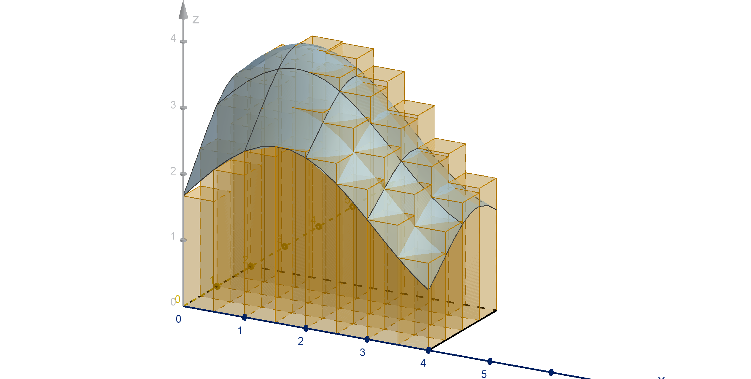
0 ≤ x ≤ 4
0 ≤ y ≤ 2
into subrectangles of area A. We
draw a prism over each rectangle
whose height is the value of the
function over some test point
(x
∗
i
, y
∗
i
).
Volume ≈
n
X
i=1
f (x
∗
i
, y
∗
i
)A.
476
Question 6.1.1
How Do We Approximate the Volume Under z = f (x, y)?
If our domain is not a rectangle, we may not be able to divide it into
subrectangles. Luckily, the formula for volume of a prism works for any
shape base. We can still compute
Volume ≈
n
X
i=1
f (x
∗
i
, y
∗
i
)A
i
.
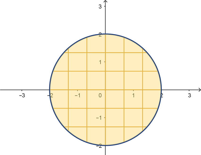
Figure: A domain subdivided into irregular subregions
477
Question 6.1.1
How Do We Approximate the Volume Under z = f (x, y)?
For a reasonably well-behaved function f (x, y), the actual volume can be
computed by taking a limit of these approximations. We call this limit
the double-integral.
Definition
Let D be a domain in R
2
. For a given division of D into n subregions
denote
A
i
, the area of the i
th
region.
(x
∗
i
, y
∗
i
), any point in the i
th
region
|A| is the diameter of the largest region.
We define the double integral of f (x, y) to be a limit over all possible
divisions of D.
ZZ
D
f (x, y)dA = lim
|A|→0
n
X
i=1
f (x
∗
i
, y
∗
i
)A
i
478
Example 6.1.2
Approximating a Double Integral
Consider
ZZ
D
x
2
ydA, where D is the region shown here. Approximate
the integral using the division of D shown, and evaluating f (x, y) at the
midpoint of each rectangle.
x
y
1
21
479
Question 6.1.3
How Do We Evaluate Double Integrals?
We already know another way of computing a volume. We can compute
the area of the cross sections perpendicular to the x-axis. Let the
function A(x) denote this area at each x. Then
Volume =
Z
b
a
A(x) dx
A(x) is itself the area under a curve. In a particular cross section, x is
constant, and f (x, y ) is a function of y . The area below this graph is the
integral
A(x) =
Z
d
c
f (x, y) dy
We can put these together to obtain an iterated integral, an integral
whose integrand is itself an integral.
480
Question 6.1.3
How Do We Evaluate Double Integrals?
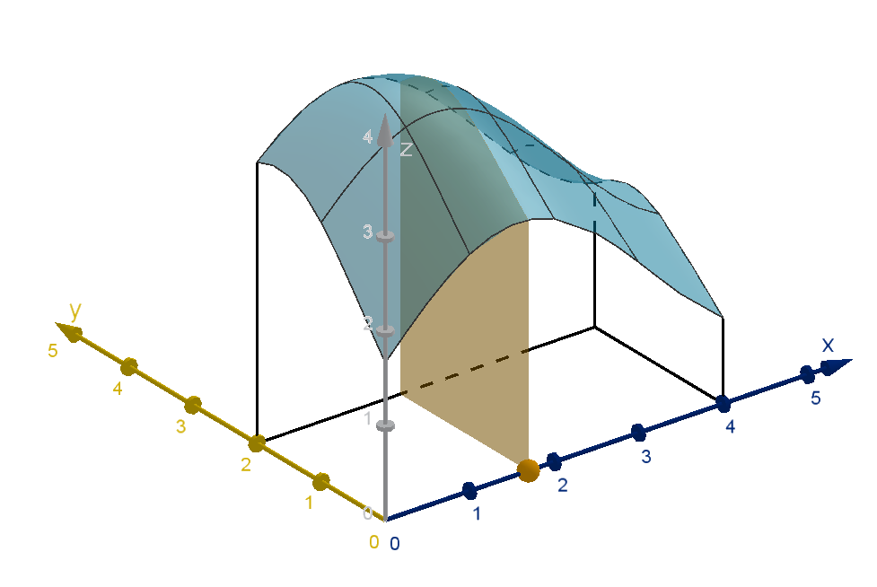
Figure: Cross sections of the region below the graph: z = f (x, y )
481
Question 6.1.3
How Do We Evaluate Double Integrals?
Theorem (Fubini’s Theorem)
For any domain D we have
ZZ
D
f (x, y) dA =
Z
b
a
Z
d
c
f (x, y) dy
dx
where a and b are the x bounds of D, and c and d are the y bounds of
the cross section at each x. Alternately, we can write
ZZ
D
f (x, y) dA =
Z
d
c
Z
b
a
f (x, y) dx
dy
where c and d are the y bounds of D, and a and b are the x bounds of
the cross section at each y.
482
Example 6.1.4
Using Fubini’s Theorem
Compute
ZZ
D
x
2
y dA, where D is the region shown here:
x
y
1
21
483
Question 6.1.5
Can We Break a Double Integral into a Product of Single Integrals?
In general, we can’t expect to factor out the inner integral of
RR
D
f (x, y)dydx (using the constant multiple rule). The y -bounds may
depend on x, and the y terms may not factor out of the integrand.
However, for certain functions and domains, this factoring is possible.
Theorem
Z
b
a
Z
d
c
f (x)g (y)dydx =
Z
b
a
f (x)dx
Z
d
c
g(y )dy
We won’t be able to use this theorem all the time. It has two important
requirements:
1 The bounds of integration (a, b, c, d) are constants. We’ll see
integrals soon where this is not the case.
2 The integrand can be factored into a function of x times a function
of y. Most two-variable functions cannot.
484
Example 6.1.6
Integrating a Product
Use a product decomposition to compute
RR
D
x
2
ydA, where D is the
region shown here:
x
y
1
21
485
Application 6.1.7
Rates (per Area)
Single integrals can compute total change given a rate of change.
meters traveled per second −→ total meters traveled.
GDP growth per year −→ total GDP growth.
mass of a chemical produced per second −→ total mass produced.
486
Application 6.1.7
Rates (per Area)
Integrating rainfall per square kilometer gives the total rain that fell in a
watershed.
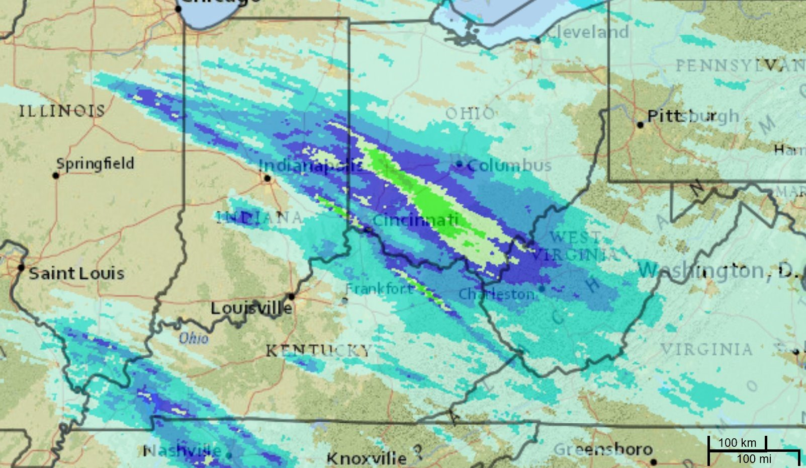
Figure: A rainfall density map
487
Application 6.1.7
Rates (per Area)
Integrating watts per square meter on a solar array gives the total energy
generated.

Figure: Solar panels
By Jud McCranie - Own work, CC BY-SA 4.0
https://commons.wikimedia.org/w/index.php?curid=70132767
488
Application 6.1.8
Probability
If we generate a data set in which we have measured two variables, then
the probability that a random data point lies in a given region is the
double integral of a joint density function over that area.
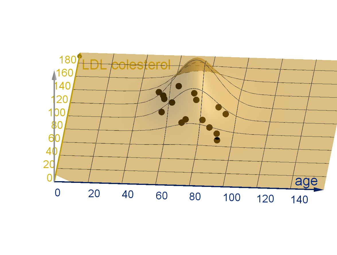
Figure: A highly correlated set of observations and an uncorrelated joint density
function
489
Section 6.1
Summary Questions
Q1 What shape do we use to approximate volume under a surface?
Q2 What formula do we use to compute the exact volume under a
graph z = f (x, y)?
Q3 What does Fubini’s Theorem tell us?
Q4 What conditions do you need in order to write a double integral as a
product of single integrals?
490
Section 6.1
Q10
Let T be the triangle with vertices (0, 0), (1, 0) and (0, 2). Show how to
approximate
ZZ
T
e
x+y
dA by dividing T into four right triangles with
legs of length 1 and
1
2
. Use the midpoint of the hypotenuses as the test
points.
491
Section 6.1
Q12
Let R be the rectangle
R = {(x, y ) : − 2 ≤ x ≤ 2, −1 ≤ y ≤ 1}.
Let S be the solid region above R and below the graph z = x
2
y + xy
2
.
Write a function A(x) which gives the area of the cross section of S
perpendicular to the x-axis at each value of x.
492
Section 6.2
Double Integrals over General Regions
Goals:
1 Set up double integrals over regions that are not rectangles.
2 Evaluate integrals where the bounds contain variables.
3 Decide when to make
R
dy the outer integral, and compute the
change of bounds.
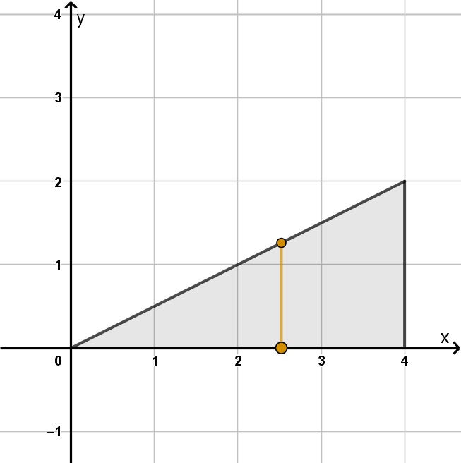
Example 6.2.1
Integrating Over a Polygon
Let D be the triangle with vertices (0, 0), (4, 0) and (4, 2). Calculate
ZZ
D
4xy dA
494
Example 6.2.1
Integrating Over a Polygon
Let D be the triangle with vertices (0, 0), (4, 0) and (4, 2). Calculate
ZZ
D
4xy dA
494
Example 6.2.1
Integrating Over a Polygon
Main Idea
To find the bounds of a double integral
1 Find the x value where the domain begins and ends. These numbers
are the bounds of the outer integral.
2 Find the functions (of the form y = g (x)) which define the top and
bottom of the domain. These functions are the bounds of the inner
integral.
495
Question 6.2.2
What Are the Integral Laws for Double Integrals?
Some single variable integral laws apply to double integrals as well
(provided the integrals exist).
1 The sum rule:
ZZ
D
f (x, y) + g (x, y )dA =
ZZ
D
f (x, y)dA +
ZZ
D
g(x, y)dA
2 The constant multiple rule:
ZZ
D
cf (x, y)dA = c
ZZ
D
f (x, y)dA
3 If D is the union of two non-overlapping subdomains D
1
and D
2
then
ZZ
D
f (x, y)dA =
ZZ
D
1
f (x, y)dA +
ZZ
D
2
f (x, y)dA
496
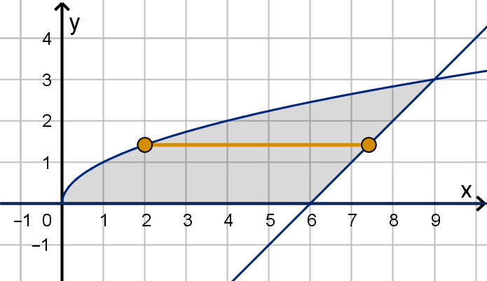
Example 6.2.3
A Region Without a (Single) Bottom Curve
Let D be the region bounded by y =
√
x, y = 0 and y = x −6. Calculate
ZZ
D
(x + y) dA.
497
Example 6.2.3
A Region Without a (Single) Bottom Curve
Let D be the region bounded by y =
√
x, y = 0 and y = x −6. Calculate
ZZ
D
(x + y) dA.
497
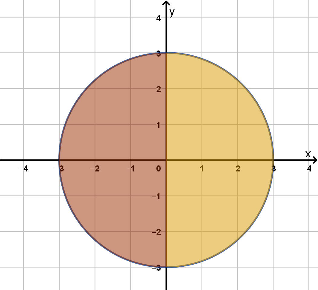
Example 6.2.4
Using Anti-Symmetry
Let D be the region x
2
+ y
2
≤ 9. Evaluate
ZZ
D
3
√
x
p
y + 3dA.
498
Example 6.2.4
Using Anti-Symmetry
Let D be the region x
2
+ y
2
≤ 9. Evaluate
ZZ
D
3
√
x
p
y + 3dA.
498
Example 6.2.4
Using Anti-Symmetry
Main Idea
We can argue that an integral
ZZ
D
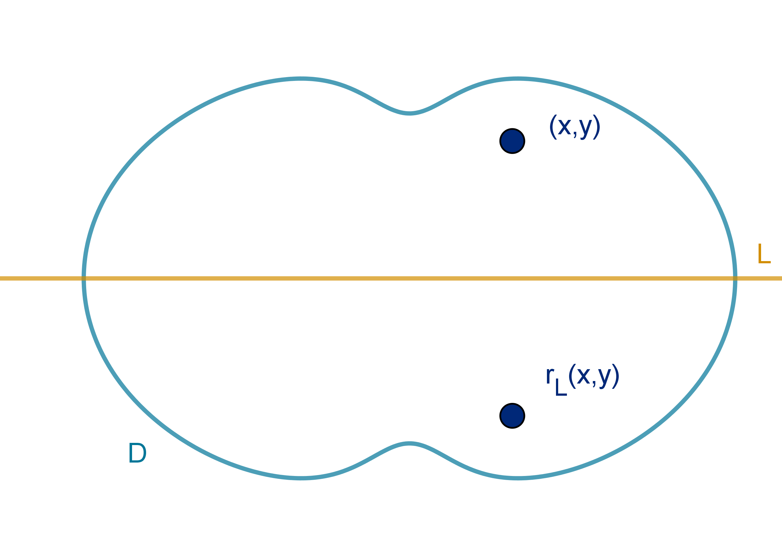
f (x, y)dA is equal to zero when
1 D is symmetric about some line L. If we folded it over L, one side
of D would lie exactly on the other side.
2 f is antisymmetric about L. For each point (x, y) in D the image
of (x, y ) across L, denoted r
L
(x, y ) has the property:
f (r
L
(x, y )) = −f (x, y ).
499
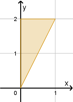
Example 6.2.5
Using Order to Manipulate the Integrand
Let D be the triangle with vertices (0, 0),
(0, 2) and (1, 2). Calculate
ZZ
D
e
(y
2
)
dA.
500
Example 6.2.5
Using Order to Manipulate the Integrand
Main Idea
If we don’t know the anti-derivative of an integrand with respect to one
variable, try switching the order of integration.
Remember to change the bounds too.
501
Application 6.2.6
Area of a Domain
Theorem
The area of a region D can be calculated:
ZZ
D
1 dA.
502
Application 6.2.6
Area of a Domain
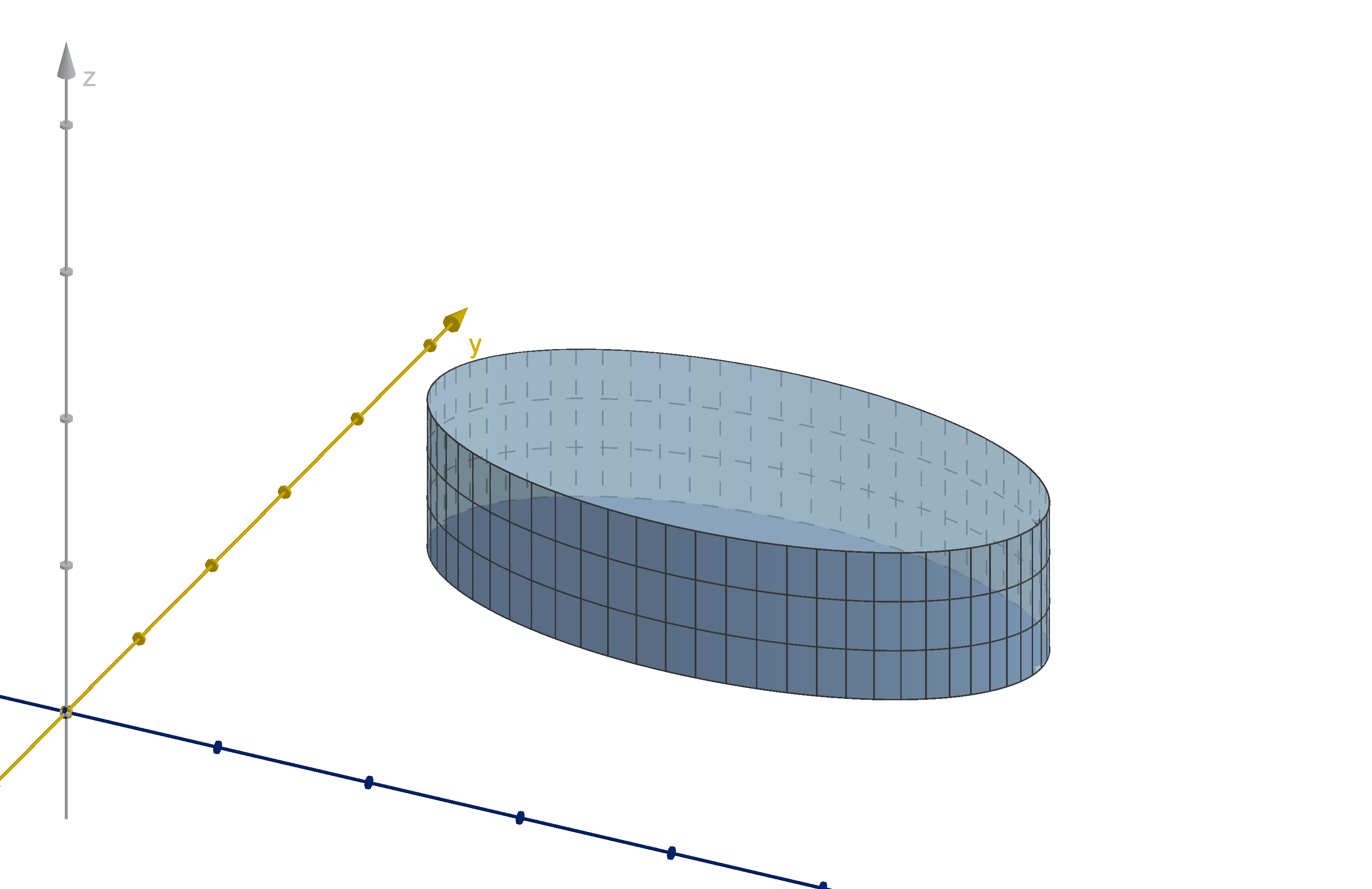
Figure: A solid of height 1 over a domain D
503
Section 6.2
Summary Questions
Q1 What are the steps for writing a double integral over a general
region?
Q2 How do you decide whether dx or dy is the inner variable?
Q3 What is antisymmetry, and how can we use it to evaluate integrals?
Q4 How can we use a double integral to compute the area of a region?
504
Section 6.2
Q8
Let D be the parallelogram with vertices (0, 1), (0, 4), (5, 3) and (5, 6).
Let f (x, y ) be a continuous function.
a Set up the bounds of integration of
ZZ
D
f (x, y) dA.
b Could we save time by computing
Z
5
0
Z
4
1
f (x, y) dydx instead?
Explain.
505
Section 6.2
Q18
Consider the integral
Z
6
−6
Z
0
−
√
36−y
2
x
2
dxdy. Write this integral in the
order dydx.
506
Section 6.2
Q20
Let g(x, y) = x
3
e
y
2
. Argue that
Z
4
−4
Z
3
−3
g(x, y) dydx = 0.
507
Section 6.2
Q24
Suppose you are given that f (x, y ) = −f (−y, −x). Over what domains
D can we argue by symmetry that
ZZ
D
f (x, y) dA = 0? Draw an
example of one.
508
Section 6.2
Q32
Consider the integral
Z
4
−4
Z
6
0
x
3
√
ydydx
a Show how to approximate the value of this integral, dividing the
domain into sub-rectangles of length 2 units and width 3 units and
using the lower right corners as test points. You should evaluate any
functions that appear in your estimate, but you do not need to
simplify the arithmetic.
b Explain in a sentence or two how you can determine the exact value
of this integral without calculating any anti-derivatives.
c Discuss what test point you could have picked in a , such that your
approximation would have computed the exact value of the integral.
Note: There are several relevant observations to make in response to
this question.
509
Section 6.3
Joint Probability Distributions
Goals:
1 Integrate a joint density function to calculate a probability.
2 Recognize when random variables are independent.
Question 6.3.1
How Do We Use Double Integrals to Compute Probabilities?
Recall how we modeled continuous random variables.
Definition
A function f is a probability density function for a random variable X ,
if the chance of an outcome a < X < b is
R
b
a
f (x)dx.
511
Question 6.3.1
How Do We Use Double Integrals to Compute Probabilities?
Definition
A pair (or more) of random variables X and Y , along with the likelihood
of various outcomes (X , Y ) is called a joint distribution. If the space of
outcomes is continuous, the distribution is modeled by a joint
probability density function f
X ,Y
(x, y ) as follows:
P(a ≤ X ≤ b and c ≤ Y ≤ d) =
Z
b
a
Z
d
c
f
X ,Y
(x, y ) dydx
More generally, for any region D in R
2
P((X , Y ) lies in D) =
ZZ
D
f
X ,Y
(x, y ) dA.
512
Example 6.3.2
Using a Joint Density Function
Suppose the random variables X and Y have the joint density function
f
X ,Y
(x, y ) =
(
x + y if 0 ≤ x ≤ 1 and 0 ≤ y ≤ 1
0 otherwise
.
Compute the probability that X is at least twice as large as Y .
513
Example 6.3.2
Using a Joint Density Function
Warning
The region of integration in this example has one fourth of the area of the
total region of possibilities, yet the answer was
5
24
not
1
4
. Do not confuse
area with probability. Not all outcomes are equally likely to occur.
Since we got a low probability, relative to area, we can deduce that the
probability density in the region we examined is lower than at some other
parts of the domain. That makes sense. The joint density function x + y
is largest in the upper right corner and lowest in the lower left. More of
our triangle was near the lower left than the upper right.
514
Example 6.3.2 Using a Joint Density Function
Exercise
Darmok and Jalad each travel to the island of Tanagra and arrive
between noon and 4 PM. Let (X , Y ) represent their respective arrival
times in hours after noon. Suppose their joint density function is
f
X ,Y
(x, y ) =
(
x
32
if 0 ≤ x ≤ 4 and 0 ≤ y ≤ 4
0 otherwise
.
1 What is the value of
R
4
0
R
4
0
f
X ,Y
(x, y )dydx?
2 Calculate the probability that Darmok arrives after 2PM.
3 Calculate the probability that Darmok arrives before Jalad.
4 What does the distribution say about when Darmok is likely to
arrive? What about Jalad?
5 Write an integral that computes the probability that they arrive
within an hour of each other (set it up, don’t evaluate).
515
Question 6.3.3
What Is a Marginal Density Function?
Recall that a density function f
X
(x) of X satisfies the property
P(a ≤ X ≤ b) =
Z
b
a
f
X
(x) dx
How can we get this function from the joint density function? We can
compute P(a ≤ X ≤ b).
P(a ≤ X ≤ b) =
Z
b
a
Z
∞
−∞
f
X ,Y
(x, y ) dydx
img/jointprobabilityaxb.pdf
516
Question 6.3.3
What Is a Marginal Density Function?
When we obtain a density function of one random variable from a joint
distribution, we call it a marginal density function.
Theorem
Given a joint distribution X , Y with joint density function f
X ,Y
, the
individual variables have marginal density functions:
f
X
(x) =
Z
∞
−∞
f
X ,Y
(x, y ) dy
f
Y
(y) =
Z
∞
−∞
f
X ,Y
(x, y ) dx
517
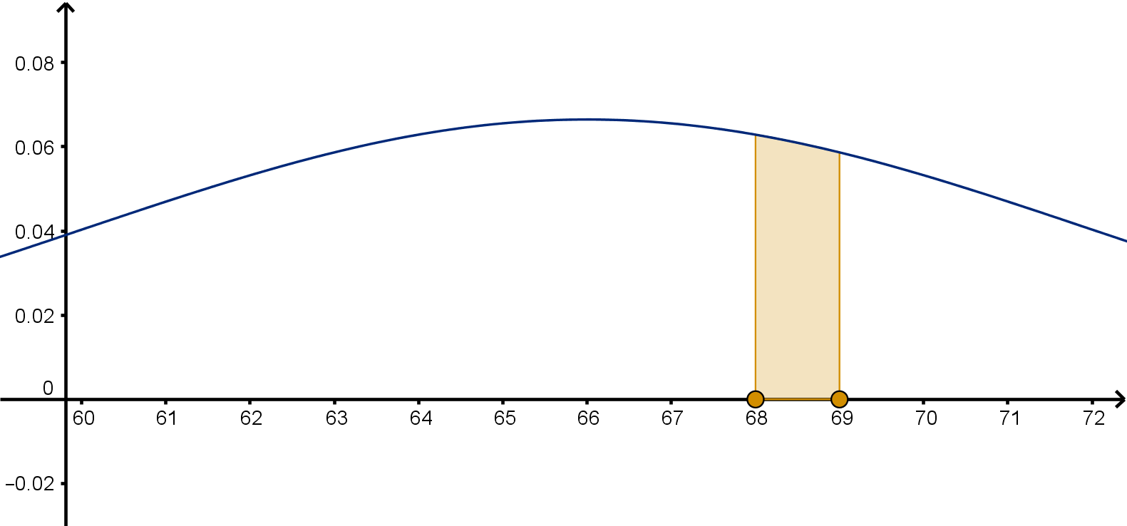
Question 6.3.3
What Is a Marginal Density Function?
For each x-value x
0
, the inner integral
Z
∞
−∞
f
X ,Y
(x
0
, y ) dy is the area of
the x = x
0
cross-section under z = f
X ,Y
(x, y ). In this figure, we see that
larger values of X are more likely, because their cross-sections have more
area.
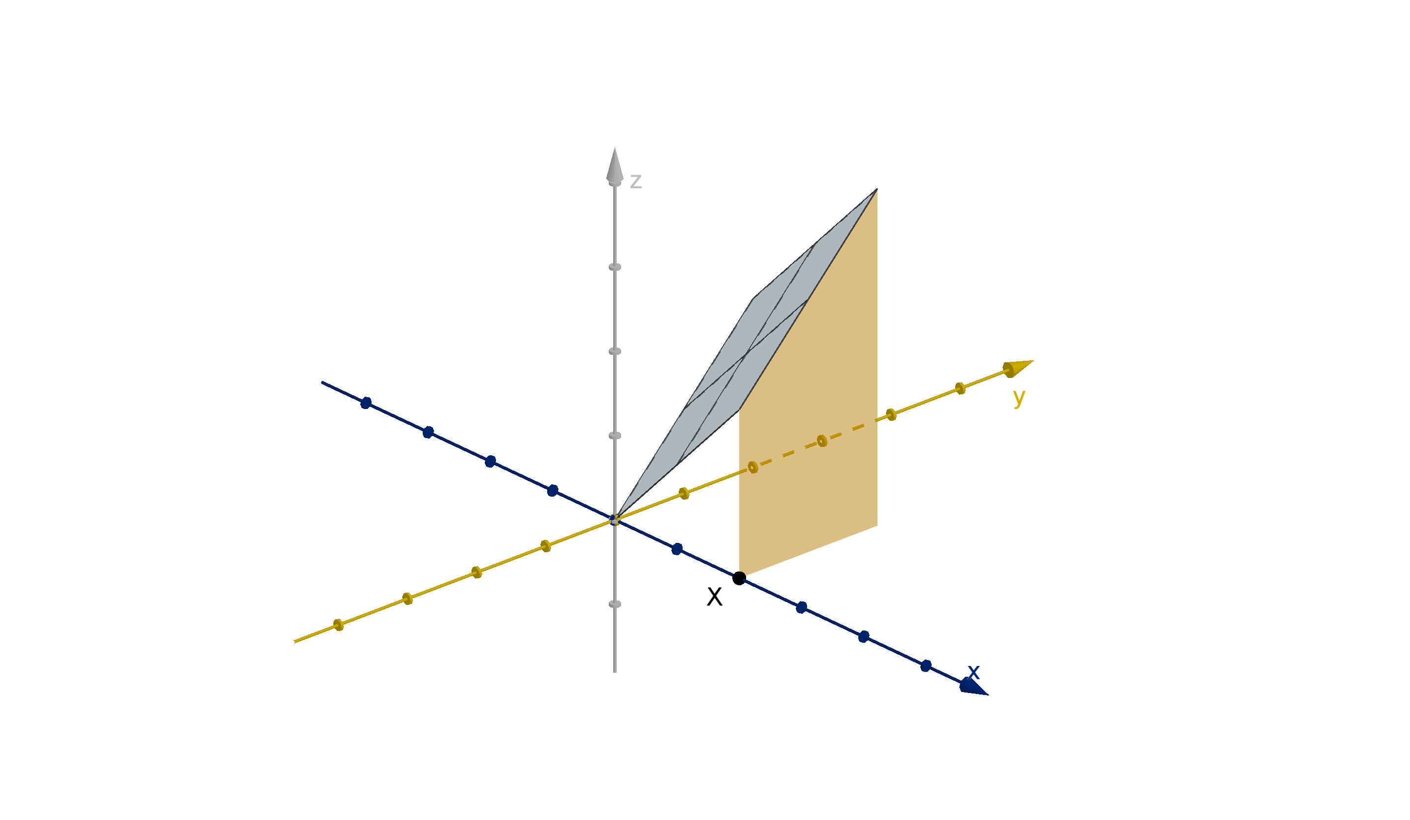
Figure: The marginal density function f
X
(x), represented as cross-sections under
z = f
X ,Y
(x, y)
518
Example 6.3.4
Computing Marginal Density Functions
Students at schools around the world compete in a rocketry contest.
Rockets are scored based on the altitude they reach (in meters). Suppose
the first and second place altitudes at a randomly chosen school are
modeled by X and Y , which have joint density function
f
X ,Y
(x, y ) =
(
12−0.012x
1000
y
x
2
−
y
2
x
3
if 0 ≤ x ≤ 1000, 0 ≤ y ≤ x
0 otherwise
a What can we infer about the possible altitudes of student rockets
from this joint density function?
b Compute the marginal density function of X , the altitude of the first
place rocket.
c What can we conclude about what values of X are more or less
likely?
519
Example 6.3.4
Computing Marginal Density Functions
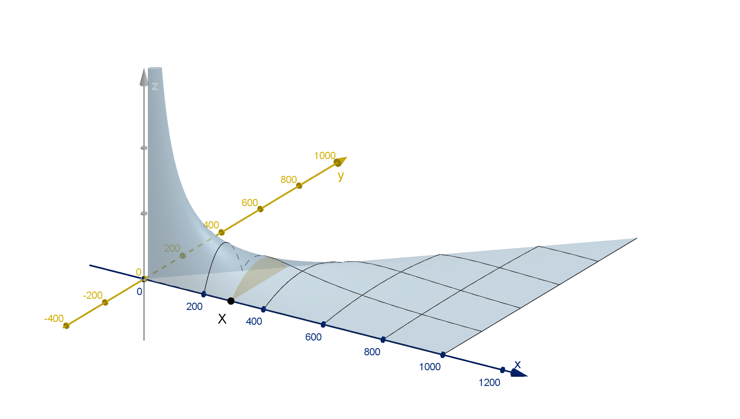
Figure: The marginal density function of X , represented as an area under the
graph of z = f
X ,Y
(x, y) (z-axis not to scale)
Remark
Even though the range of possible outcomes is greater for larger X , the
probability of achieving that X is smaller. We can see this in the cross
sections on the joint-density function. Larger values of X have longer
cross sections, but it is the area under the graph z = f
X ,Y
(x, y ) that
matters.
520
Example 6.3.4
Computing Marginal Density Functions
Main Idea
If the range of possible outcomes is limited, then computing f
X
(x)
requires us to:
1 make different computations for different ranges of X and
2 within each computation, divide the integral into pieces depending
on which values of Y are possible.
521
Question 6.3.5
Why Do We Need Joint Distributions?
In some cases we don’t.
Definition
If the outcomes of Y don’t depend on the outcome of X and vice versa,
we say X and Y are independent. In this case
P(a ≤ X ≤ b and c ≤ Y ≤ d) =
Z
b
a
f
X
(x) dx
Z
d
c
f
Y
(y) dy
522
Question 6.3.5
Why Do We Need Joint Distributions?
Example
Suppose Darmok and Jalad’s arrival times have the joint density function
f
X ,Y
(x, y ) =
(
x
32
if 0 ≤ x ≤ 4 and 0 ≤ y ≤ 4
0 otherwise
.
Jalad’s arrival time is uniformly distributed. Darmok’s is triangular.
Neither distribution depends on the arrival time of the other.
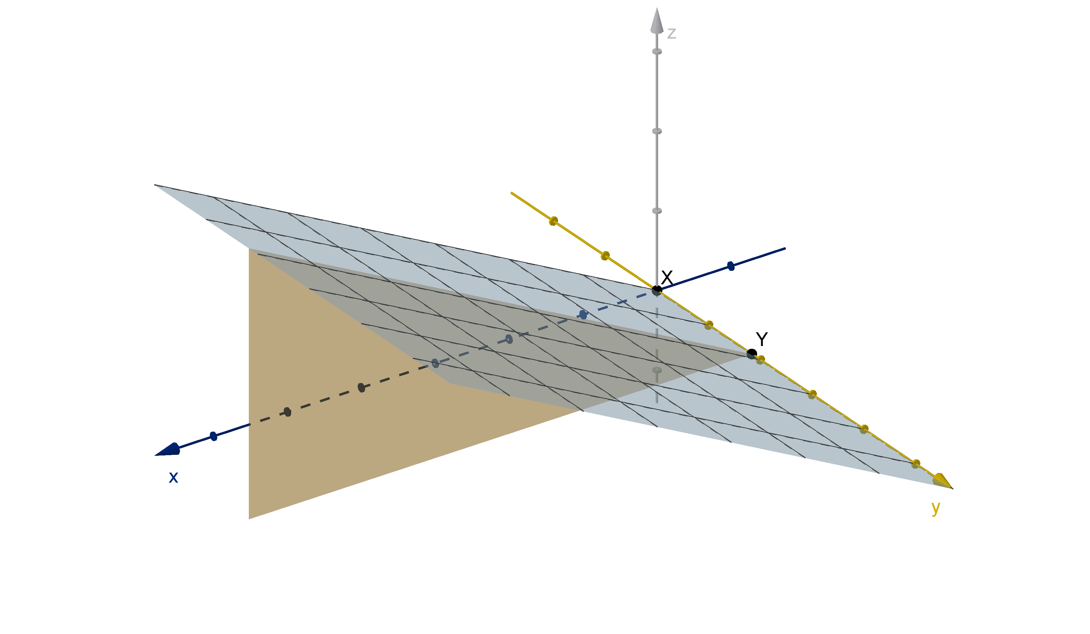
Figure: The density function for Darmok and Jalad’s arrival times
523
Question 6.3.5
Why Do We Need Joint Distributions?
Theorem
X and Y are independent, if and only if their joint density function can
be written f
X ,Y
(x, y ) = g (x)h(y), where
g(x) is a function only of x
h(y ) is a function only of y
Remark
g(x) and h(y ) can be chosen to be the marginal density functions of X
and Y , but they don’t need to be. As long as a factorization exists, the
variables are independent.
524
Question 6.3.5
Why Do We Need Joint Distributions?
Example
Suppose
f
X ,Y
(x, y ) =
(
3π
12π−8
cos
π
2
x
(2y − y
2
) if 0 ≤ x ≤ 6 and 0 ≤ y ≤ 4
0 otherwise
f
X ,Y
(x, y ) factors into the marginal density functions
f
X
(x) =
(
π
3π−2
cos
π
2
x
if 0 ≤ x ≤ 6
0 otherwise
f
Y
(y) =
(
3
4
(2y − y
2
) if 0 ≤ y ≤ 4
0 otherwise
Thus we can conclude that X and Y are independent.
525
Question 6.3.5
Why Do We Need Joint Distributions?
We can see independence in the cross sections of z = f
X ,Y
(x, y ).
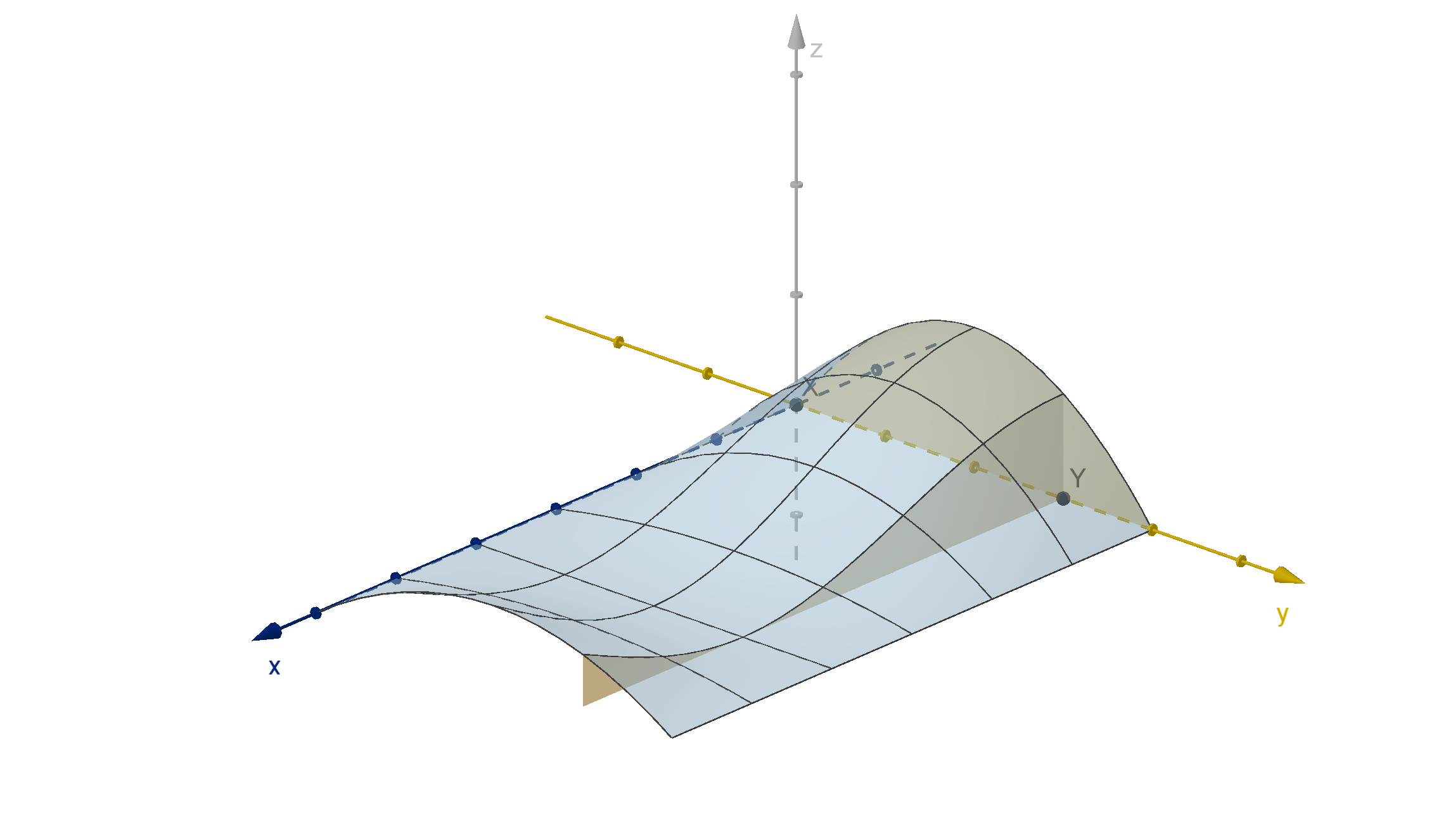
Figure: An independent joint density function and its cross sections
526
Question 6.3.6
What Is the Expected Value of a Function of X and Y?
What if we wanted to know the expected value the function
g(X , Y ) =
Y
2
X
? By definition, this is very hard. We would need to write
a density function h(t) such that
Z
b
a
h(t) dt = P
a ≤
Y
2
X
≤ b
Notice g(x, y) = a and g (x, y ) = b are level curves of g . In this case
they solve to
x =
1
a
y
2
x =
1
b
y
2
527
Question 6.3.6
What Is the Expected Value of a Function of X and Y?
In the case of Darmok and Jalad, the probabilities that h(t) produces
would have to integrate to give the probability that (X , Y ) lies between
the level curves:
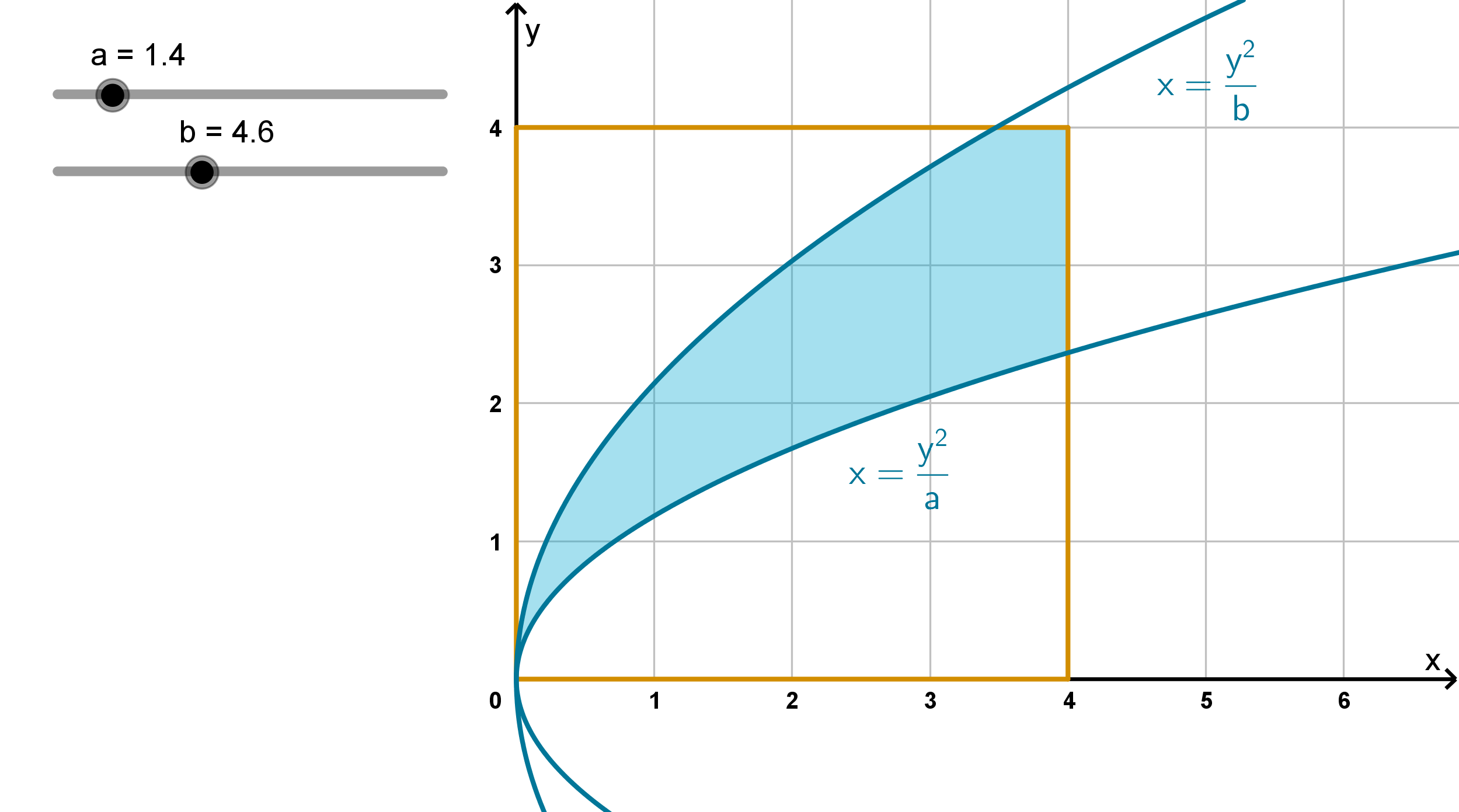
Figure: The region where a ≤ g(x, y) ≤ b
528
Question 6.3.6
What Is the Expected Value of a Function of X and Y?
Computing expected values of functions by producing a new density
function would be intractable. Fortunately there is a multivariable
analogue to the expected value theorem from single variable density
functions.
Theorem
The expected value of a function g(X , Y ) of two continuous random
variables X and Y with joint density function f
X ,Y
(x, y ) can be
computed:
E [g(X )] =
Z
∞
−∞
Z
∞
−∞
g(x, y)f
X ,Y
(x, y ) dydx.
529
Example 6.3.7
Expected Value of a Random Variable
A special case of the expected value formula is to compute the expected
values of g(x, y) = x or g (x, y ) = y . Suppose X and Y have joint
density function
f
X ,Y
(x, y ) =
(
12−0.012x
1000
y
x
2
−
y
2
x
3
if 0 ≤ x ≤ 1000, 0 ≤ y ≤ x
0 otherwise
Compute E [X ].
530
Example 6.3.7
Expected Value of a Random Variable
Main Ideas
We can compute E [X ] or E [Y ] by integrating
E [X ] =
Z
∞
−∞
Z
∞
−∞
xf
X ,Y
(x, y ) dydx
E [Y ] =
Z
∞
−∞
Z
∞
−∞
yf
X ,Y
(x, y ) dydx
If we already have the marginal density function f
X
(x) (or f
Y
(y)),
we can use the single-variable expected value formula:
E [X ] =
Z
∞
−∞
xf
X
(x) dx
In fact, we saw this integral partway through our solution.
Computing the marginal density function is nearly equivalent to
computing the inner integral in the two-variable expected value
formula.
531
Example 6.3.8
Expected Value of a Function
Compute the expected value of
Y
2
X
where X is Darmok’s arrival time and
Y is Jalad’s arrival time. Assume that X and Y have joint density
function:
f
X ,Y
=
(
x
32
if 0 ≤ x ≤ 4 and 0 ≤ y ≤ 4
0 otherwise
.
532
Application 6.3.9
Average Value of a Function
Definition
The uniform distribution over a region D in R
2
has the joint density
function
f
X ,Y
=
(
1
area of D
if (x, y ) is inside D
0 if (x, y ) is outside D
533
Application 6.3.9
Average Value of a Function
Like with single variable function, we default to the uniform distribution
whenever we average a function and no specific random variable is
specified.
Definition
The average value of a function f over a region D is defined to be the
expected value of f (X , Y ) where X , Y are uniformly distributed over D.
f
ave
=
1
Area of D
ZZ
D
f (x, y) dA
Since we can also compute the area of D using a double integral, we can
also write
f
ave
=
RR
D
f (x, y) dA
RR
D
1 dA
534
Application 6.3.10
Covariance and Correlation
Definition
The expected value of (X −E [X ])(Y −E [Y ]) is called the covariance of
X and Y , denoted cov(X , Y ).
1 If cov(X , Y ) > 0, higher values of X tend to be correlated with
higher values of Y .
2 If cov(X , Y ) < 0, higher values of X tend to be correlated with
lower values of Y .
3 If cov(X , Y ) = 0, X and Y are uncorrelated.
535
Application 6.3.10
Covariance and Correlation
Suppose X and Y are independent. Then outcomes of X should not
depend on outcomes of Y . The joint density function can be written
f (x, y) = g (x)h(y). We can use our integral rules to see that covariance
is always 0, matching our intuition.
cov(X , Y ) =
Z
∞
−∞
Z
∞
−∞
(x − E[X ])(y − E[Y ])f
X ,Y
(x, y ) dydx
=
Z
∞
−∞
Z
∞
−∞
(x − E[X ])(y − E[Y ])g(x)h(y ) dydx
=
Z
∞
−∞
(x − E[X ])g(x) dx
Z
∞
−∞
(y − E[Y ])h(y ) dy
=
Z
∞
−∞
xg(x) dx − E [X ]
Z
∞
−∞
yh(y ) dy − E[Y ]
= (0)(0)
536
Application 6.3.10
Covariance and Correlation
A joint distribution could have a large covariance because the variables
are consistently correlated, or because X (or Y ) has high variance
(meaning X is generally farther from E [X ]). To control for the latter
effect we often compute:
Pearson’s Correlation
ρ
X ,Y
=
cov(X , Y )
σ
X
σ
Y
Where the σs are standard deviations.
ρ returns a value between −1 and 1 which is one measure of how
well-correlated two random variables are.
537
Section 6.3
Summary Questions
Q1 How do we use a joint density function to compute the probability
of a certain set of outcomes?
Q2 What is a marginal density function and how do we compute it?
Q3 What does it mean for two random variables to be independent?
Q4 How can we tell from the graph of a joint density function that the
two random variables are independent?
538
Section 6.3
Q20
How does the distribution of Y change as X takes different values, given
the following joint density function?
f
X ,Y
(x, y ) =
(
x + y if 0 ≤ x ≤ 1 and 0 ≤ y ≤ 1
0 otherwise
Are X and Y independent?
539
Section 6.3
Q22
f
X ,Y
(x, y ) is a joint density function for a pair of independent variables X
and Y . Here is a picture of the x = 2 cross section of z = f
X ,Y
(x, y ).
a Describe what values of Y are more or less likely when X = 2.
b Assume f
X ,Y
(x, y ) is not always 0 at x = 5. Describe what values of
Y are more or less likely when X = 5.
c How is the shape of the x = 2 cross section of z = f
X ,Y
(x, y )
related to the x = 5 cross section of z = f
X ,Y
(x, y )?
540
Section 6.4
Triple Integrals
Goals:
1 Set up triple integrals over three-dimensional domains.
2 Evaluate triple integrals.
Question 6.4.1
How Do We Integrate a Three-Variable Function?
Definition
Given a domain D in three dimension space, and a function f (x, y, z).
We can subdivide D into regions
V
i
is the volume of the i
th
region.
(x
∗
i
, y
∗
i
, z
∗
i
) is a point in the i
th
region.
V is the diameter of the largest region.
We define the triple integral of f over D to be the following limit over
all possible divisions of D:
ZZZ
D
f (x, y, z) dV = lim
V →0
n
X
i=1
f (x
∗
i
, y
∗
i
, z
∗
i
)V
i
542
Question 6.4.1
How Do We Integrate a Three-Variable Function?
Fubini’s theorem applies to triple integrals as well. We write them as
iterated integrals.
Theorem
ZZZ
D
f (x, y, z)dV =
Z
x
2
x
1
Z
y
2
y
1
Z
z
2
z
1
f (x, y, z) dzdydx
where
z
1
and z
2
are the bounds of z, which may be functions of x and y .
y
1
and y
2
are the bounds of y, which may be functions of x.
x
1
and x
2
are the bounds of x. They are numbers.
The variables of can also be reordered, with the bounds defined
analogously.
543
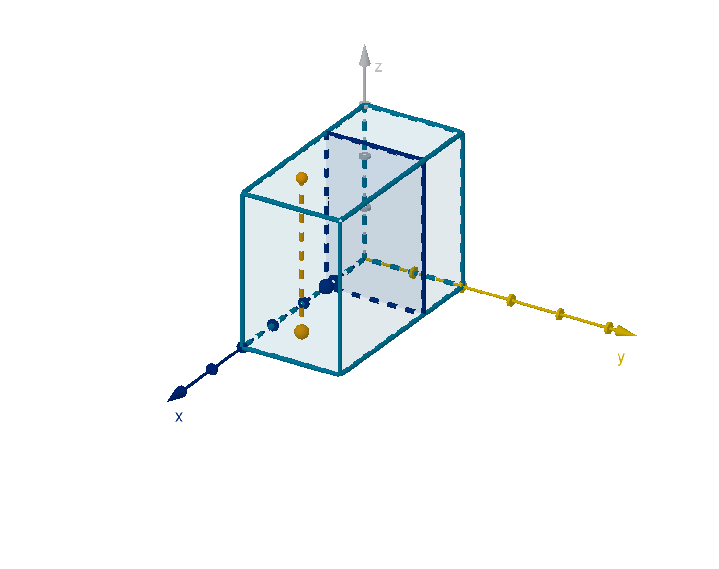
Example 6.4.2
Integrating Over a Prism
Let R = {(x, y , z) : 0 ≤ x ≤ 4, 0 ≤ y ≤ 2, 0 ≤ z ≤ 3}. Compute
ZZZ
R
3zy + x
2
dV .
544
Example 6.4.2
Integrating Over a Prism
Let R = {(x, y , z) : 0 ≤ x ≤ 4, 0 ≤ y ≤ 2, 0 ≤ z ≤ 3}. Compute
ZZZ
R
3zy + x
2
dV .
Figure: A Rectangular Prism
544
Question 6.4.3
How Do We Interpret Triple Integrals Geometrically?
Z
3
0
f (x, y, z) dz computes the area under the graph w = f (x, y, z) over
each vertical segment of the form (x, y ) = (x
0
, y
0
) in the domain. It is a
function of x and y .
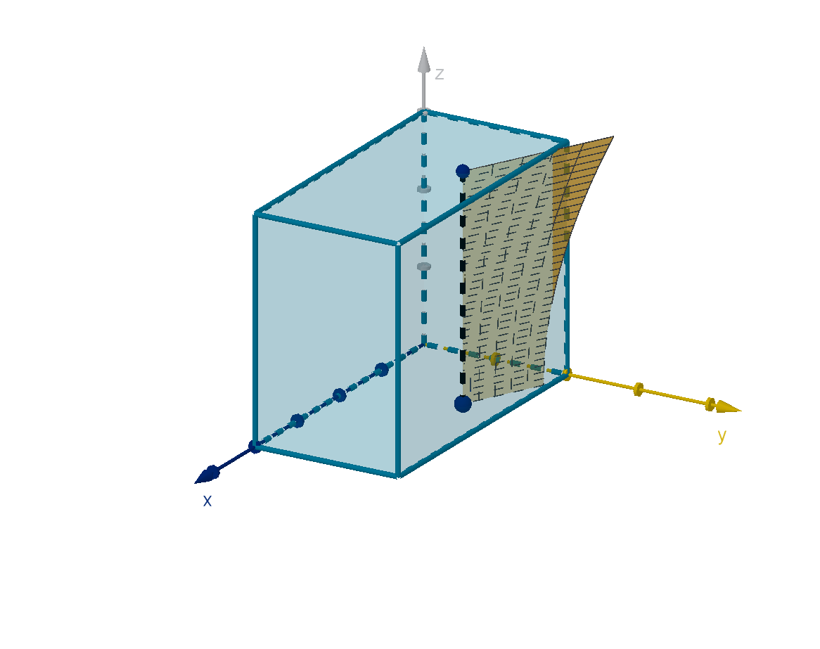
Figure:
Z
3
0
f (x, y, z) dz, represented as an area in a zw -plane
545
Question 6.4.3
How Do We Interpret Triple Integrals Geometrically?
Z
2
0
Z
3
0
f (x, y, z) dzdy computes the volume under the graph
w = f (x, y, z) over each x = x
0
cross-section of the domain. It is a
function of x.
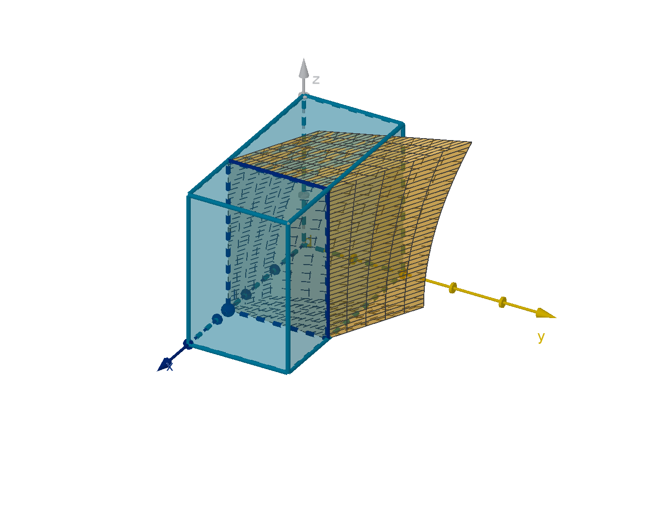
Figure:
Z
2
0
Z
3
0
f (x, y, z) dzdy, represented as a volume in yzw-space
546
Application 6.4.4
Triple Integrals in Math and Science
1 Integrating a function ρ(x, y , z), which gives the density of an object
at each point, gives the total mass of the object.
2 Integrating xρ(x, y , z), y ρ(x, y, z) and zρ(x, y, z) gives the center
of mass of the object.
3 Integrating a three-dimensional probability distribution over a region
gives the probability that the triple (X , Y , Z ) lies in that region.
4 Integrating 1 dV over a region gives the volume of that region.
547
Application 6.4.4
Triple Integrals in Math and Science
Density lets us visualize a triple integral without referring to a fourth
(geometric) dimension.
Z
3
0
f (x, y, z) dz computes
the density of the vertical
segments at each (x, y ).
Z
2
0
Z
3
0
f (x, y, z) dzdy
computes the density of the
rectangle at each x.
Z
4
0
Z
2
0
Z
3
0
f (x, y, z) dzdydx computes the total mass of the prism.
548
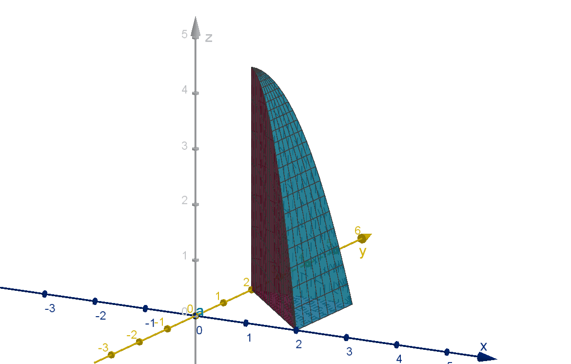
Example 6.4.5
Integrating Over an Irregular Region
Let R be the region above the xy plane, below the cylinder x
2
+ z
2
= 16
and between y = 0 and y = 3. Compute
ZZZ
R
4yz dV .
549
Example 6.4.5
Integrating Over an Irregular Region
Let R be the region above the xy plane, below the cylinder x
2
+ z
2
= 16
and between y = 0 and y = 3. Compute
ZZZ
R
4yz dV .
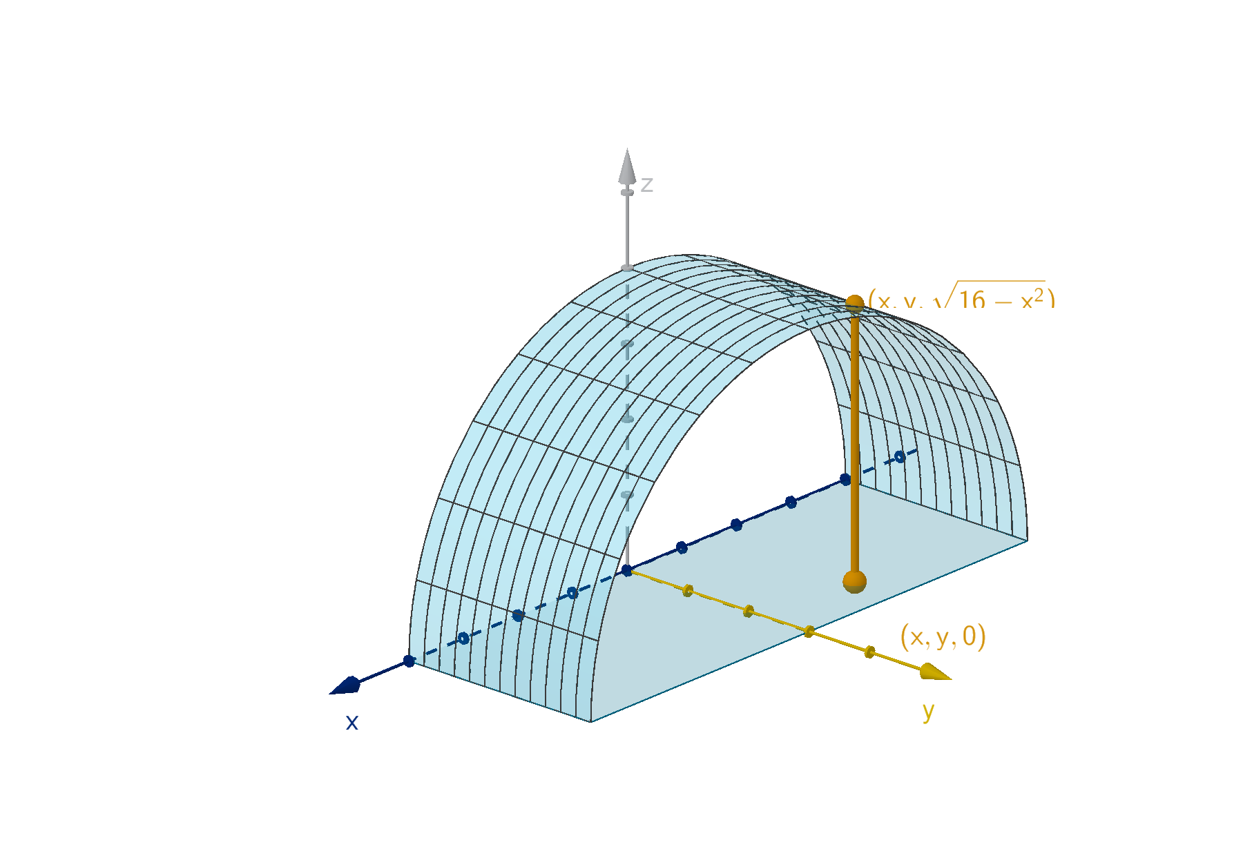
Figure: The region between x
2
+ y
2
= 16 and the xy -plane
549
Example 6.4.5
Integrating Over an Irregular Region
Main Idea
The following approach will produce the bounds of a region with a top
surface and a bottom surface.
1 The z bounds are given by the equations z = f (x, y ) and
z = g(x, y ) of the top and bottom surface.
2 The intersection of the top and bottom surface can produce relevant
bounds on x and y. We can graph these, along with any given
bounds involving x and y.
3 After drawing the bounded region in the xy-plane, the x and y
bounds are computed as for a double integral.
Like with double integrals, we will want to break the region into smaller
pieces in some cases. In other cases, we may want to change the order of
integration.
550
Example 6.4.6
A Solid Given by Vertices
Suppose we want to integrate over T , the tetrahedron (pyramid) with
vertices (0, 0, 0), (4, 0, 0), (4, 2, 0) and (4, 0, 2). How would we set up the
bounds of integration?
551
Example 6.4.6
A Solid Given by Vertices
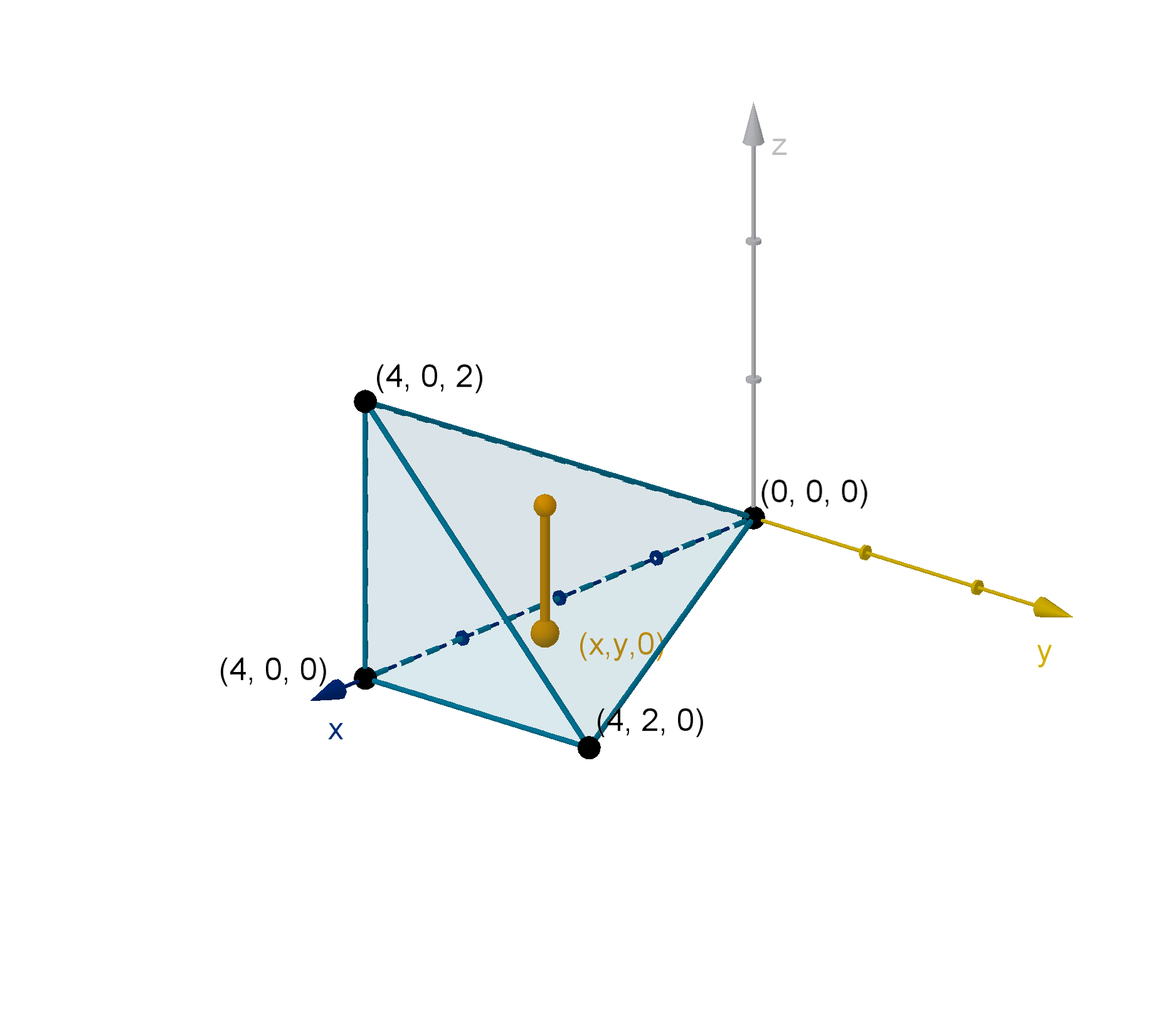
Figure: z bounds of T
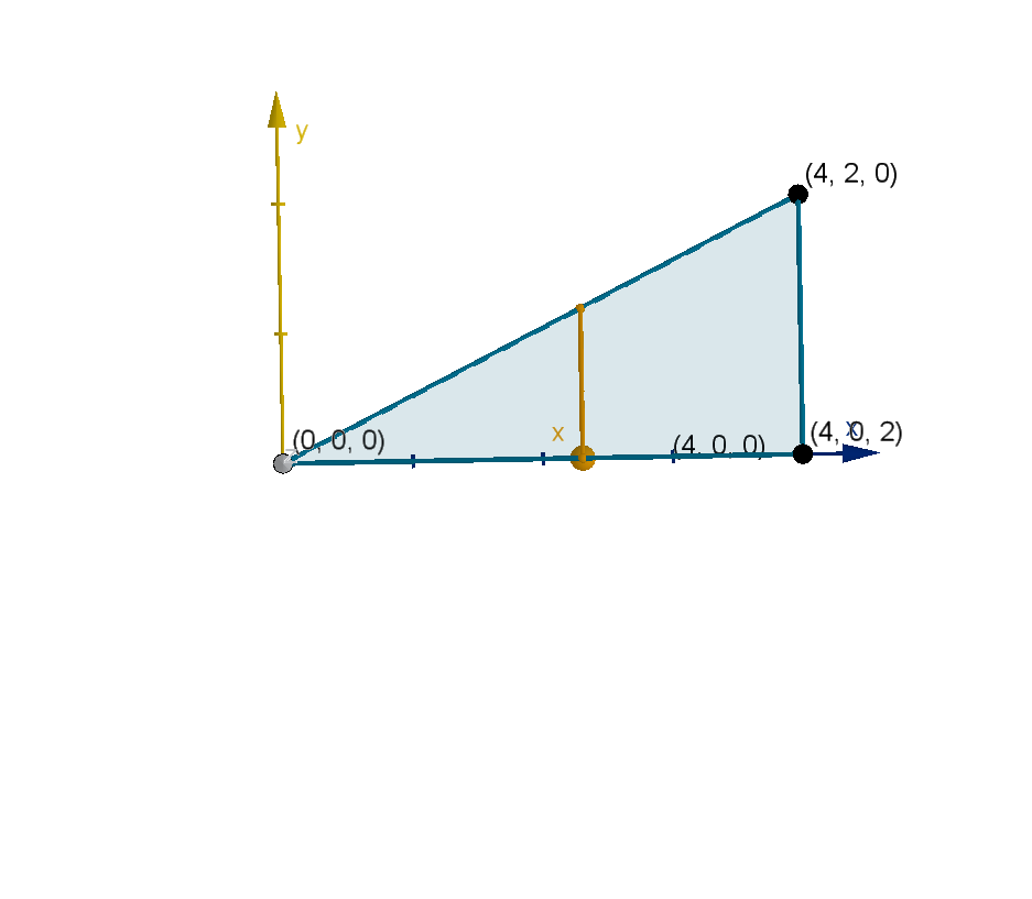
Figure: x, y bounds of T
552
Example 6.4.7
Changing the Order of Integration
Suppose D is the bounded region enclosed between the graph of
y = 4x
2
+ z
2
and the plane y = 4. Set up the bounds of the integral
ZZZ
D
f (x, y, z)dV .
Figure: A region bounded by a paraboloid and a plane
553
Example 6.4.7
Changing the Order of Integration
Suppose D is the bounded region enclosed between the graph of
y = 4x
2
+ z
2
and the plane y = 4. Set up the bounds of the integral
ZZZ
D
f (x, y, z)dV .
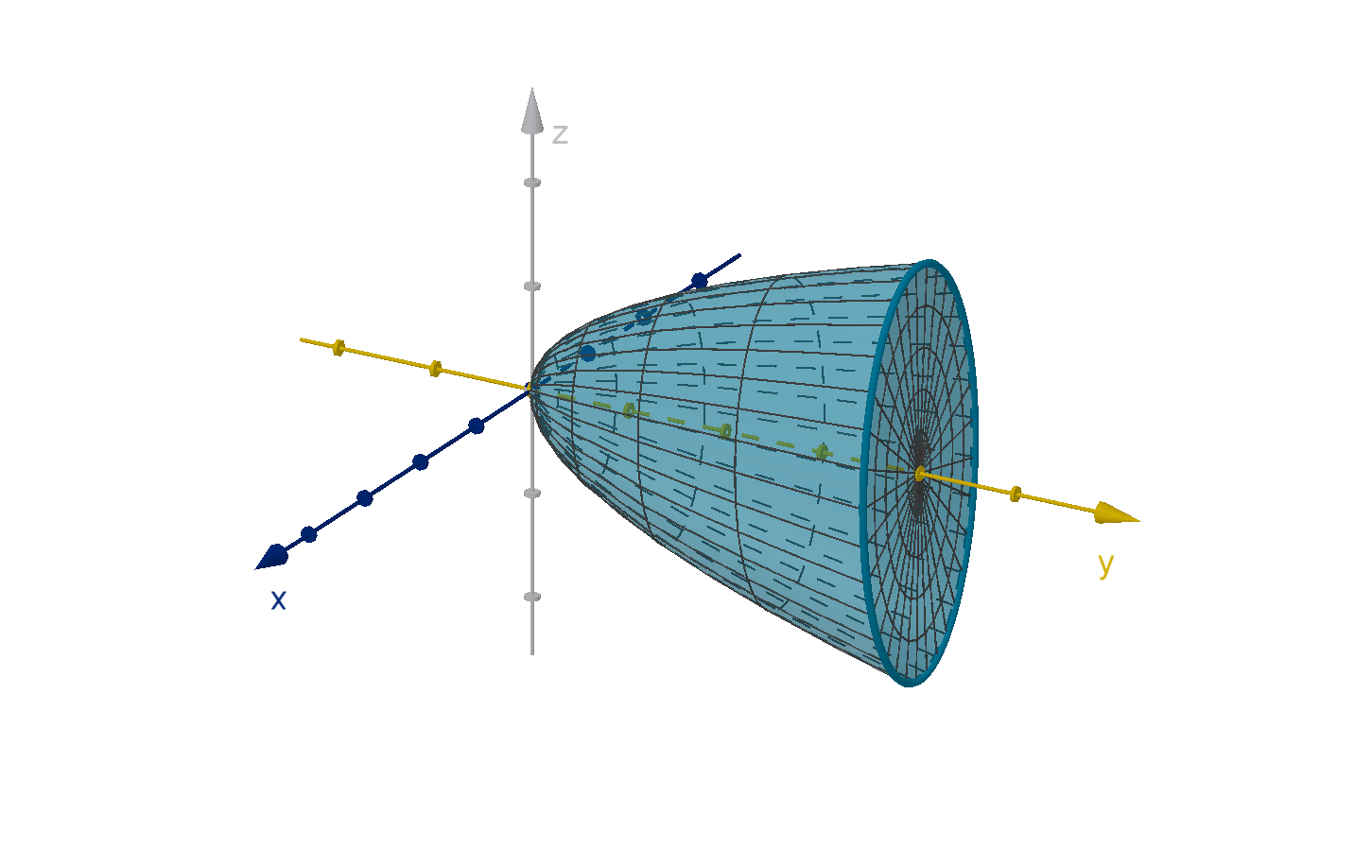
Figure: A region bounded by a paraboloid and a plane
553
Question 6.4.8
When Does a Triple Integral Decompose as a Product?
The product theorem from double integrals also works here:
Theorem
If y
1
, y
2
, z
1
and z
2
are constants, then
Z
x
2
x
1
Z
y
2
y
1
Z
z
2
z
1
f (x)g (y)h(z) dzdydx
=
Z
x
2
x
1
f (x) dx
Z
y
2
y
1
g(y ) dy
Z
z
2
z
1
h(z) dz
554
Question 6.4.8
When Does a Triple Integral Decompose as a Product?
Example
Along with the sum and constant multiple rules we can simplify
Z
4
0
Z
2
0
Z
3
0
3zy + x
2
dzdydx
to obtain the following:
Z
4
0
Z
2
0
Z
3
0
3zy dzdydx +
Z
4
0
Z
2
0
Z
3
0
x
2
dzdydx
=3
Z
4
0
dx
Z
2
0
y dy
Z
3
0
z dz +
Z
4
0
x
2
dx
Z
2
0
dy
Z
3
0
dz
=3 ·4
Z
2
0
y dy
Z
3
0
z dz + 2 · 3
Z
4
0
x
2
dx
555
Section 6.4
Summary Questions
Q1 What does Fubini’s theorem say about integrals with dV ?
Q2 How is density used to understand triple integrals. Why wasn’t it
necessary or appropriate for double integrals?
Q3 How do you find the bounds of the inner variable in a triple integral?
Q4 How to you find the bounds of the other two variables?
556
Section 6.4
Q26
Let R be the region enclosed by y =
√
25 −x
2
, z = 6 −y and z =
√
y.
Set up the bounds of
RRR
R
g(x, y, z)dV .
557
Section 6.4
Q26
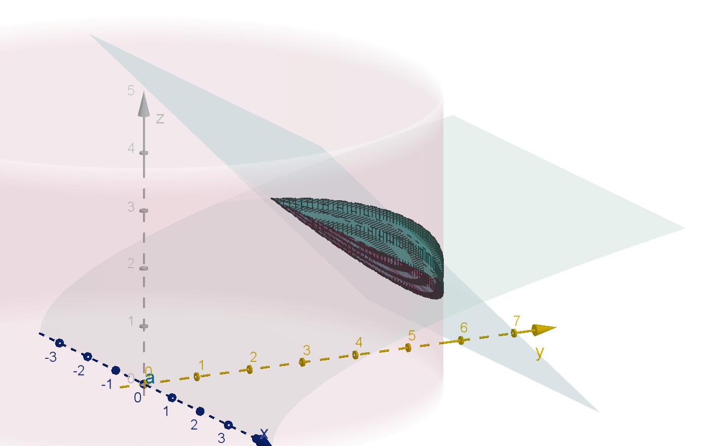
Figure: The region enclosed by x
2
+ y
2
= 25, z = 6 −y, and z =
√
y
558
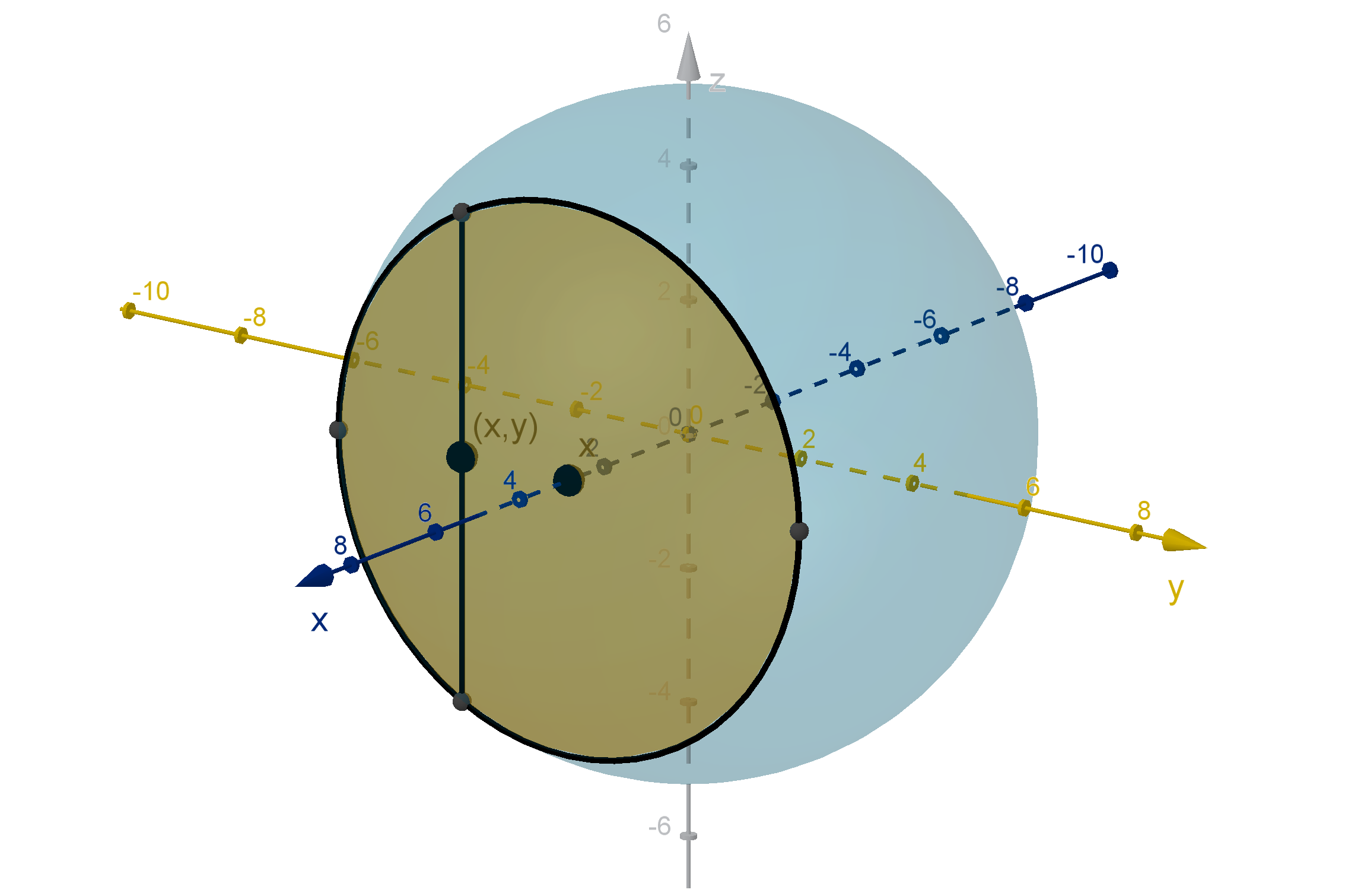
Section 6.4
Q20
Cheng is integrating over R, the region given by x
2
+ y
2
+ z
2
≤ 25. He
gives the following setup. Is this valid?
Z
√
25−y
2
−z
2
−
√
25−y
2
−z
2
Z
√
25−x
2
−z
2
−
√
25−x
2
−z
2
Z
√
25−x
2
−y
2
−
√
25−x
2
−y
2
f (x, y, z) dzdydx
559
Section 6.4
Q20
559
Section 6.4
Q22
Let R = {(x, y , z) : z ≤ 2x − y, z ≥ 0, y ≥ x
2
}. Compute
ZZZ
R
xz dV .
560
Section 6.4
Q36
Rewrite the integral
Z
2
0
Z
2
2−x
Z
4−x
2
0
f (x, y, z) dzdydx as an integral with
the differential dxdzdy.
561
Section 6.4
Q36
562
Section 6.4
Q38
Let S = {(x, y, z) : x
2
+ y
2
+ z
2
≤ 25}. Explain why
ZZZ
S
x
3
y
4
cos πz dV cannot be decomposed as a product.
563