Section 5.1
Vectors
Goals:
1 Distinguish vectors from scalars (real numbers) and points.
2 Add and subtract vectors, multiply by scalars.
3 Express real world vectors in terms of their components.
Question 5.1.1
What is a Vector?
Definition
A vector in 2-space consists of a magnitude (length) and a direction.
Two vectors with the same magnitude and the same direction are equal.
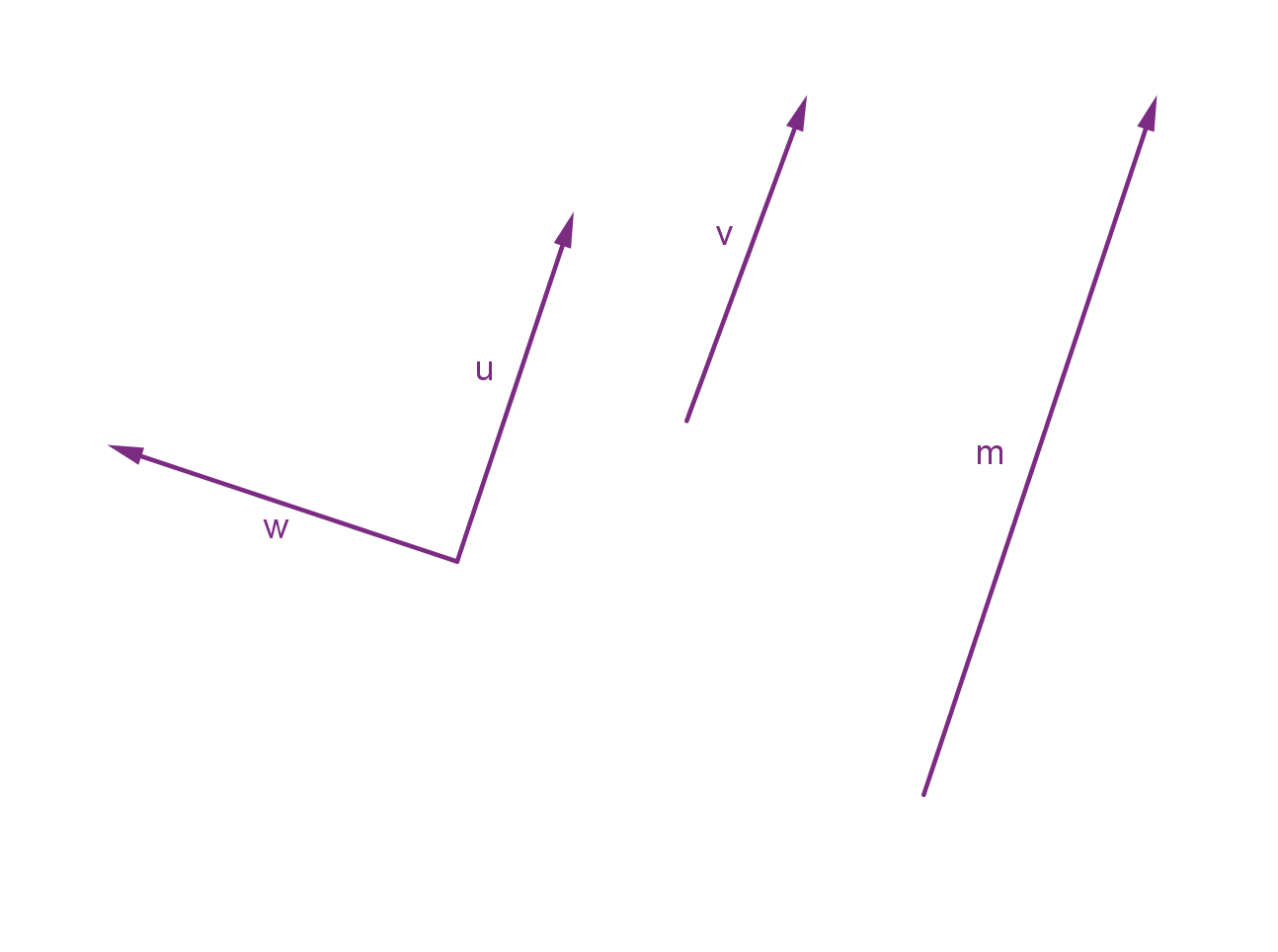
Example
Here are four vectors in 2-space (the plane) represented by arrows. Two
of these vectors are equal.
335
Question 5.1.1
What is a Vector?
Here are some vectors
3 miles south
The force that a magnetic field applies to a charged particle
The velocity of an airplane
Here are some non-vectors
17
The mass of an automobile
3:15 PM
Atlanta, GA
336
Question 5.1.2
How Do We Denote Vectors?
Endpoint Notation
The vector
v from point A to point B can be represented by the notation
−→
AB.
A is the initial point and B is the terminal point.
337
Question 5.1.2
How Do We Denote Vectors?
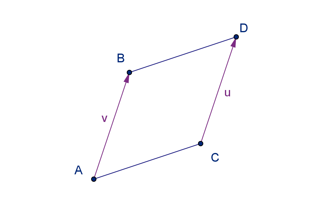
Theorem
−→
AB =
−→
CD if and only if ABDC is a parallelogram (perhaps a squished
one).
338
Question 5.1.2
How Do We Denote Vectors?
Coordinate Notation
We can represent a vector in the Cartesian plane by the x and y
components of its displacement. If A = (2, 3) and B = (5, 1), then
−→
AB
increases x by 5 − 2 = 3 and y by 1 − 3 = −2. We can represent
−→
AB = ⟨3, −2⟩
Figure: The x and y components of a vector
339
Question 5.1.2
How Do We Denote Vectors?
Theorem
v =
u if and only if their coordinate representations match in each
component.
We can also measure slope using the coordinate notation. For the vector
v = ⟨a, b⟩:
b represents the displacement in the y-direction (rise).
a represents the displacement in the x-direction (run).
The slope of
v is
rise
run
=
b
a
.
340
Question 5.1.2
How Do We Denote Vectors?
Every point in a Cartesian coordinate system has a position vector,
which gives the displacement of that point from the origin. The
components of the vector are the coordinates of the point.
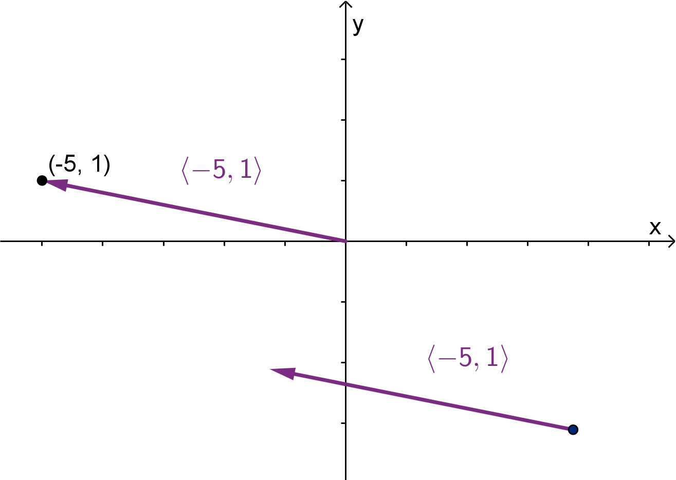
Figure: There is only one point equal to (−5, 1), but there are many vectors
equal to ⟨−5, 1⟩.
341
Question 5.1.3
What Arithmetic Can We Perform with Vectors?
Vector Sums
The sum of two vectors
v +
u is calculated by positioning
v and
u head
to tail. The sum is the vector from the initial point of one to the
terminal point of the other. In coordinate notation, we just add each
component numerically.
⟨ 1, 3⟩
+⟨ 3, −1⟩
⟨ 4, 2⟩
342
Question 5.1.3
What Arithmetic Can We Perform with Vectors?
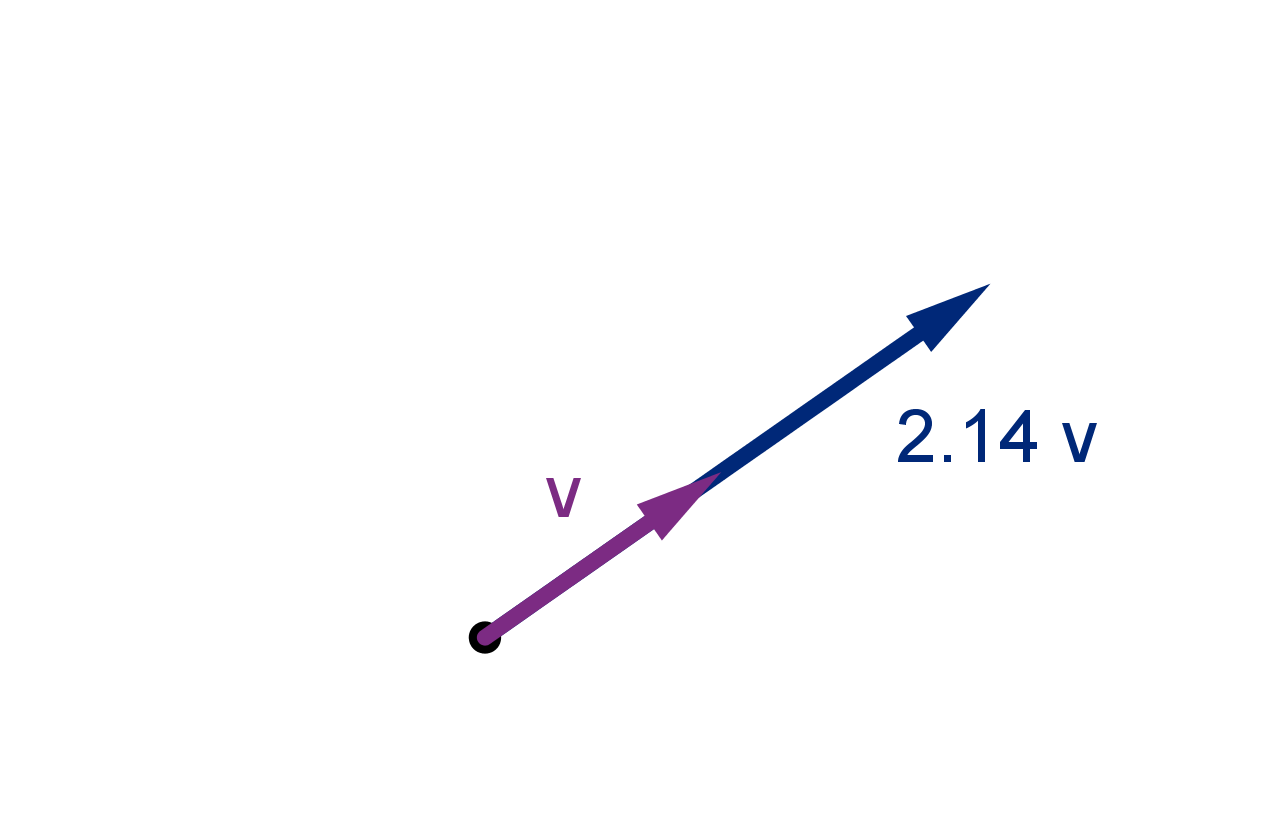
Scalar Multiples
Given a number (called a scalar) λ and a vector
v we can produce the
scalar multiple λ
v, which is the vector in the same direction as
v but λ
times as long.
If λ is negative then λ
v extends in
the opposite direction. Either way,
we say λ
v is parallel to
v.
In coordinates scalar multiplication is distributed to each component. For
example:
2.5 ⟨6, 4⟩ = ⟨15, 10⟩
343
Example 5.1.4
Performing Vector Arithmetic
Given diagrams of two vectors
u and
v, how would we calculate
1
2
u +
v?
What if we are instead given the components
u = ⟨a, b⟩ and
v = ⟨c, d⟩?
344
Question 5.1.5
What Is Standard Basis Notation?
We can represent any vector in the plane as a sum of scalar multiples of
the following standard basis vectors.
Standard Basis Vectors
The emphstandard basis vectors in R
2
are
i = ⟨1, 0⟩
j = ⟨0, 1⟩
For example, the vector ⟨3, −5⟩ can be written as 3
i − 5
j. You can check
yourself that the sum on the right gives the correct vector.
345
Question 5.1.6
How Do We Measure the Length of a Vector?
Definition
The length or magnitude of a vector is calculated using the distance
formula and notated |
v|. If
v = a
i + b
j, then
|
v| =
p
a
2
+ b
2
346
Example 5.1.7
The Length of a Vector
If
v = ⟨3, −5⟩ calculate |
v|
347
Example 5.1.7
The Length of a Vector
Definition
A unit vector is a vector of length 1. Given a vector
v the scalar multiple
1
|
v|
v
is a unit vector in the same direction as
v.
348
Question 5.1.8
How Do We Measure the Direction of a Vector?
Angles are a good way of comparing directions. In general, two vectors
will not intersect to form an angle, so we use the following definition:
Definition
The angle between two vectors is the angle they make when they are
placed so their initial points are the same.
If they make a right angle, we call them orthogonal. If they make an
angle of 0 or π, they are parallel.
349
Question 5.1.9
How Do We Denote Vectors in Higher Dimensions?
Higher dimensional vectors represent displacements in higher dimensional
spaces. We can call a vector in n-space an n-vector. We can still denote
and n-vector by its endpoints. We can also denote it in coordinate
notation, but we need more components.
Example
If A = (2, 4, 1) and B = (5, −1, 3) then
−→
AB = ⟨3, −5, 2⟩.
350
Question 5.1.9
How Do We Denote Vectors in Higher Dimensions?
In three space, we add another standard basis vector
k.
Standard basis for 3-vectors
i = ⟨1, 0, 0⟩
j = ⟨0, 1, 0⟩
k = ⟨0, 0, 1⟩
Example
⟨3, −5, 2⟩ = 3
i − 5
j + 2
k
Higher dimensions still have a standard basis, but at this point the
naming conventions are less standard. {
e
1
,
e
2
,
e
3
, . . . ,
e
n
} is common for
n-vectors.
351
Question 5.1.9
How Do We Denote Vectors in Higher Dimensions?
Length of a Vector
The length of an n-vector derives from the distance formula in n-space.
|⟨a
1
, a
2
, a
3
, . . . , a
n
⟩| =
q
a
2
1
+ a
2
2
+ a
2
3
+ ···+ a
2
n
352
Question 5.1.9
How Do We Denote Vectors in Higher Dimensions?
Angles Between Vectors
Any two vectors with the same initial point lie in a plane. Their angle is
a two-dimensional measurement.
However there is no good way to measure clockwise in 3 or more
dimensions. The angle between two vectors is never negative, nor more
than π.
353
Question 5.1.9
How Do We Denote Vectors in Higher Dimensions?
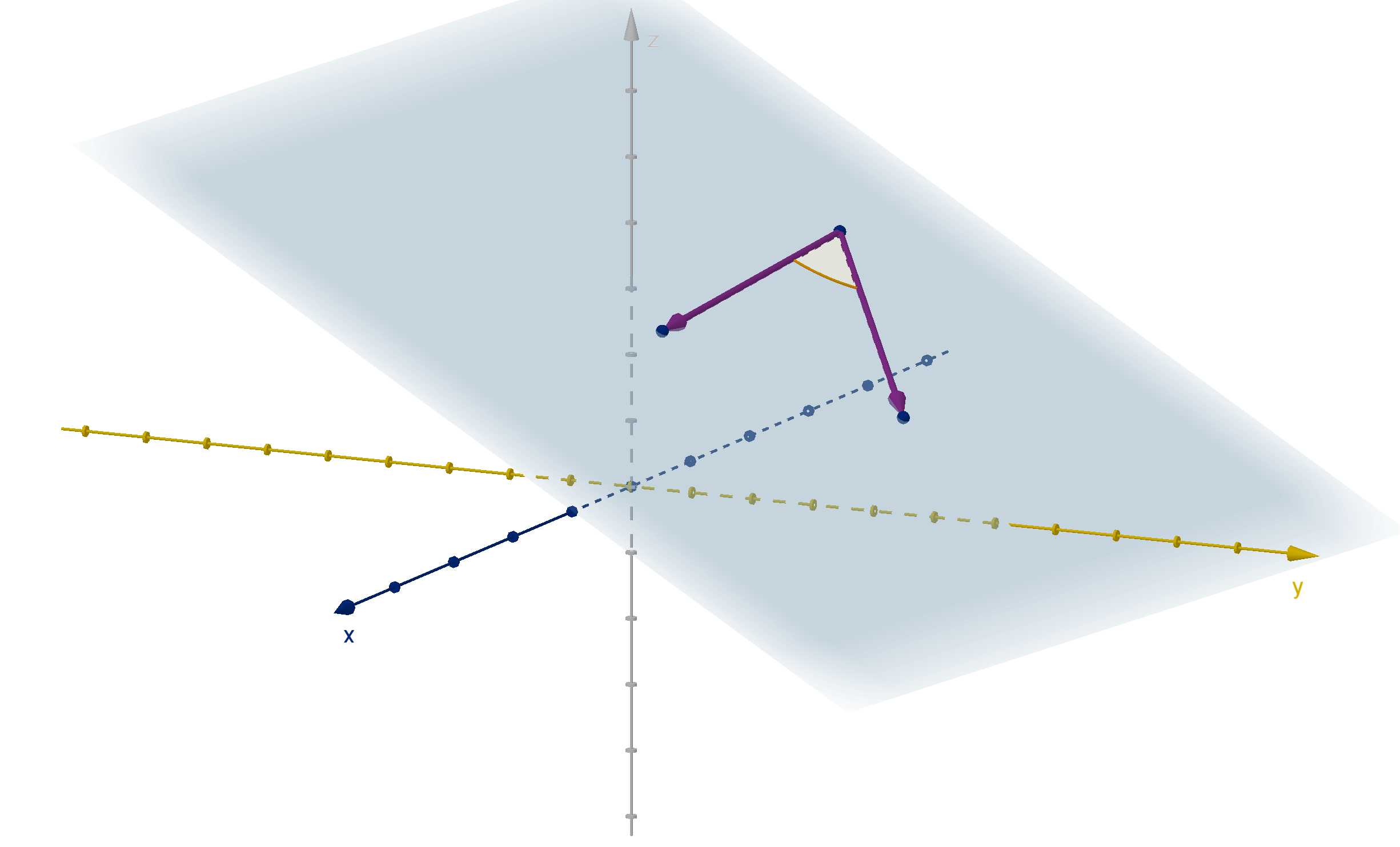
Figure: Two 3-vectors with a common initial point, the plane that contains
them, and the angle between them
354
Section 5.1
Summary Questions
Q1 How is a vector similar to a point? To a number?
Q2 How is a vector different from a point? From a number?
Q3 How can you tell if two vectors point in the same direction?
Opposite directions?
Q4 If
u and
v are position vectors of the points P and Q, how are
u
and
v related to
−→
PQ?
355
Section 5.1
Q42
Let
u and
v be non-parallel vectors in R
3
. How many unit vectors in R
3
are orthogonal to both
u and
v?
356
Section 5.2
The Dot Product
Goals:
1 Calculate the dot product of two vectors.
2 Determine the geometric relationship between two vectors based on
their dot product.
3 Calculate vector and scalar projections of one vector onto another.
Question 5.2.1
What Is the Dot Product?
Definition
The dot product of two vectors is a number.
For two dimensional vectors
v = ⟨v
1
, v
2
⟩ and
u = ⟨u
1
, u
2
⟩ we define
v ·
u = v
1
u
1
+ v
2
u
2
For three dimensional vectors
v = ⟨v
1
, v
2
, v
3
⟩ and
u = ⟨u
1
, u
2
, u
3
⟩ we
define
v ·
u = v
1
u
1
+ v
2
u
2
+ v
3
u
3
This pattern can be extended to any dimension.
358
Example 5.2.2
Computing a Dot Product
a Calculate ⟨2, 3, −1⟩ · ⟨4, 1, 5⟩
b Calculate (−2
i + 4
k) ·(
i + 2
j −
k)
359
Question 5.2.3
What Are the Algebraic Properties of the Dot Product?
Theorem
The following algebraic properties hold for any vectors
u,
v and
w and
scalars m and n.
Commutative
u ·
v =
v ·
u
Distributive
u ·(
v +
w) =
u ·
v +
u ·
w
Associative m
u ·n
v = mn(
u ·
v)
360
Question 5.2.4
What Is the Geometric Significance of the Dot Product?
Theorem
If
u and
v are parallel then
u ·
v =
(
|
u||
v| if
u and
v have the same direction
−|
u||
v| if
u and
v have opposite directions
361
Question 5.2.4
What Is the Geometric Significance of the Dot Product?
Theorem
If
u and
v are orthogonal then
u ·
v = 0.
362
Question 5.2.4
What Is the Geometric Significance of the Dot Product?
Two vectors need not be parallel or orthogonal, but given vectors
u and
v we can always write
v =
v
proj
+
v
orth
.
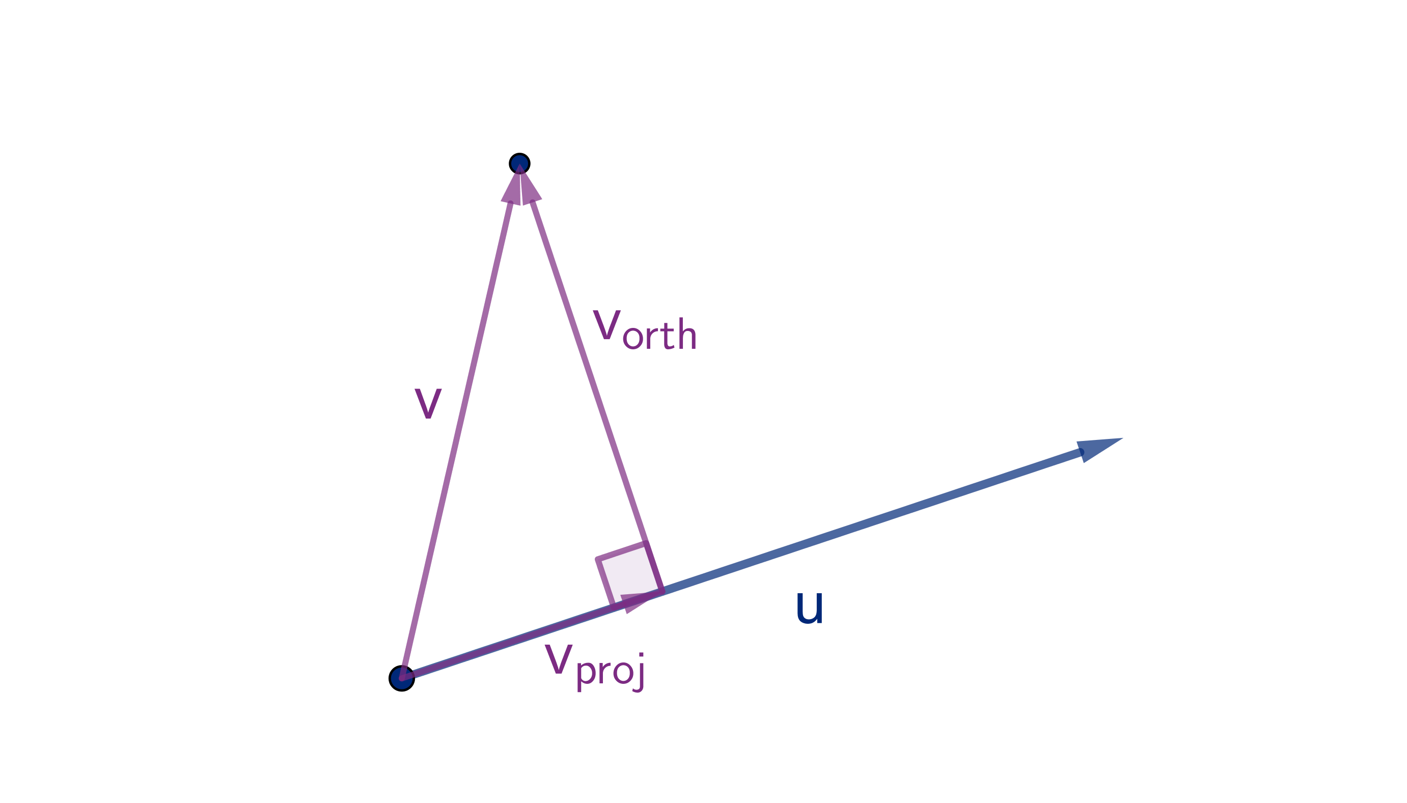
The properties of the dot
product tell us that
u ·
v =
u ·(
v
proj
+
v
orth
)
= ±|
u||
v
proj
| + 0
Definition
The number
u ·
v
|
u|
is called the
scalar projection of
v onto
u.
363
Question 5.2.4
What Is the Geometric Significance of the Dot Product?
Theorem
Let
u and
v have the same initial point and meet at angle θ. The
following formula holds in any dimension:
u ·
v = |
u||
v|cos θ
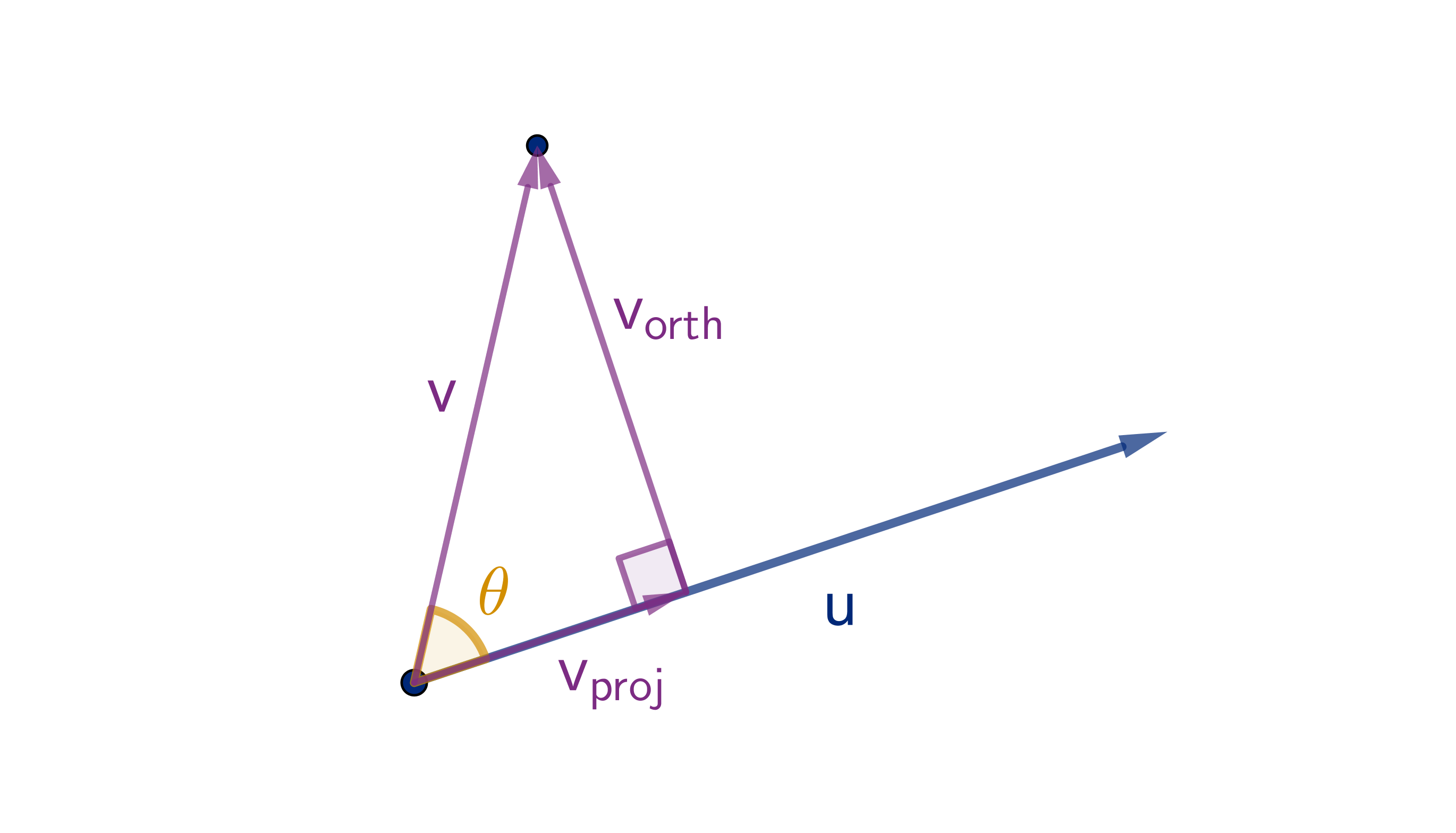
Recall that cos θ is
positive when θ < π/2
negative when θ > π/2
zero when θ = π/2.
So the sign of
u ·
v tells us
whether θ is acute, obtuse or
right.
364
Example 5.2.5
Using the Cosine Formula
What is the angle between ⟨1, 0, 1⟩ and ⟨1, 1, 0⟩?
365
Example 5.2.5
Using the Cosine Formula
What is the angle between ⟨1, 0, 1⟩ and ⟨1, 1, 0⟩?
365
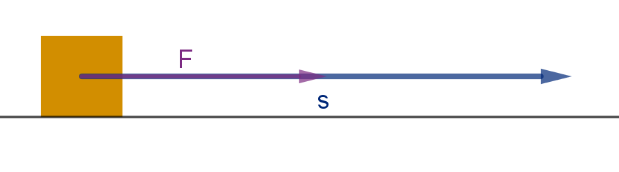
Application 5.2.6
Work
In physics, we say a force works on an object if it moves the object in
the direction of the force. Given a force F and a displacement s, the
formula for work is:
W = Fs
366
Application 5.2.6
Work
In higher dimensions, displacement and force are vectors.
If the force and the displacement are not in the same direction, then only
F
proj
contributes to work.
W =
F
proj
·
s =
F ·
s
367
Section 5.2
Summary Questions
Q1 What algebraic properties does a dot product share with real
number multiplication?
Q2 What is the significance of the dot product of two parallel vectors?
Q3 How is the angle between two vectors related to their dot product?
Q4 What is a scalar projection, and how do you compute it?
368
Section 5.2
Q16
If |
u| = 6 and |
v| = 10 what are the greatest and least possible values of
u ·
v?
369
Section 5.2
Q16
If |
u| = 6 and |
v| = 10 what are the greatest and least possible values of
u ·
v?
370
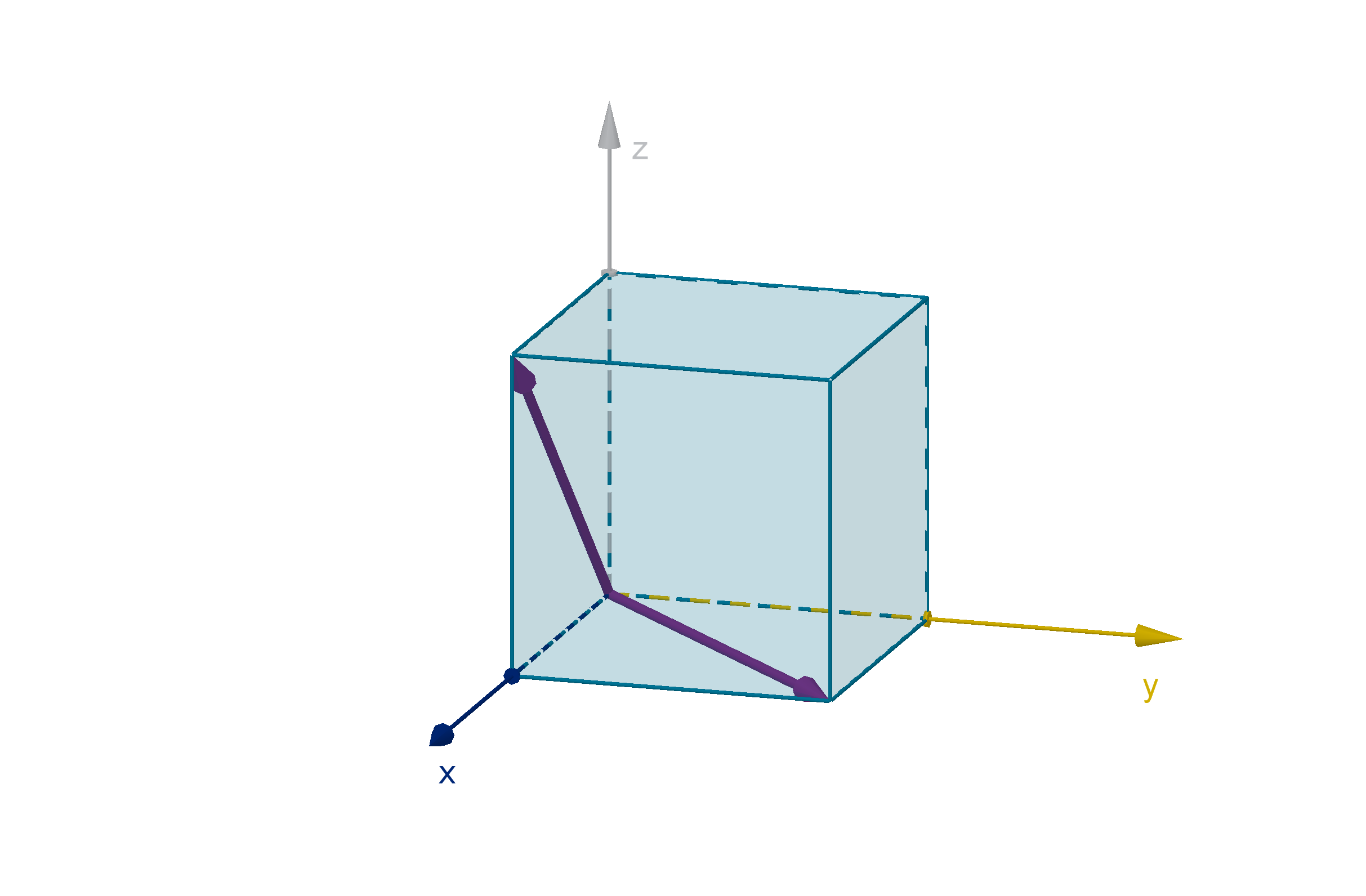
Section 5.2
Q22
Let A be the vertex of a cube, and B and C be any two other points on
the cube. Use a dot product to explain why the angle between
−→
AB and
−→
AC cannot be larger than
π
2
. (Hint, put A at (0, 0, 0).)
371
Section 5.3
Normal Equations of Planes
Goals:
1 Give equations of planes in both vector and normal forms.
2 Use normal vectors to measure the distance to a plane.
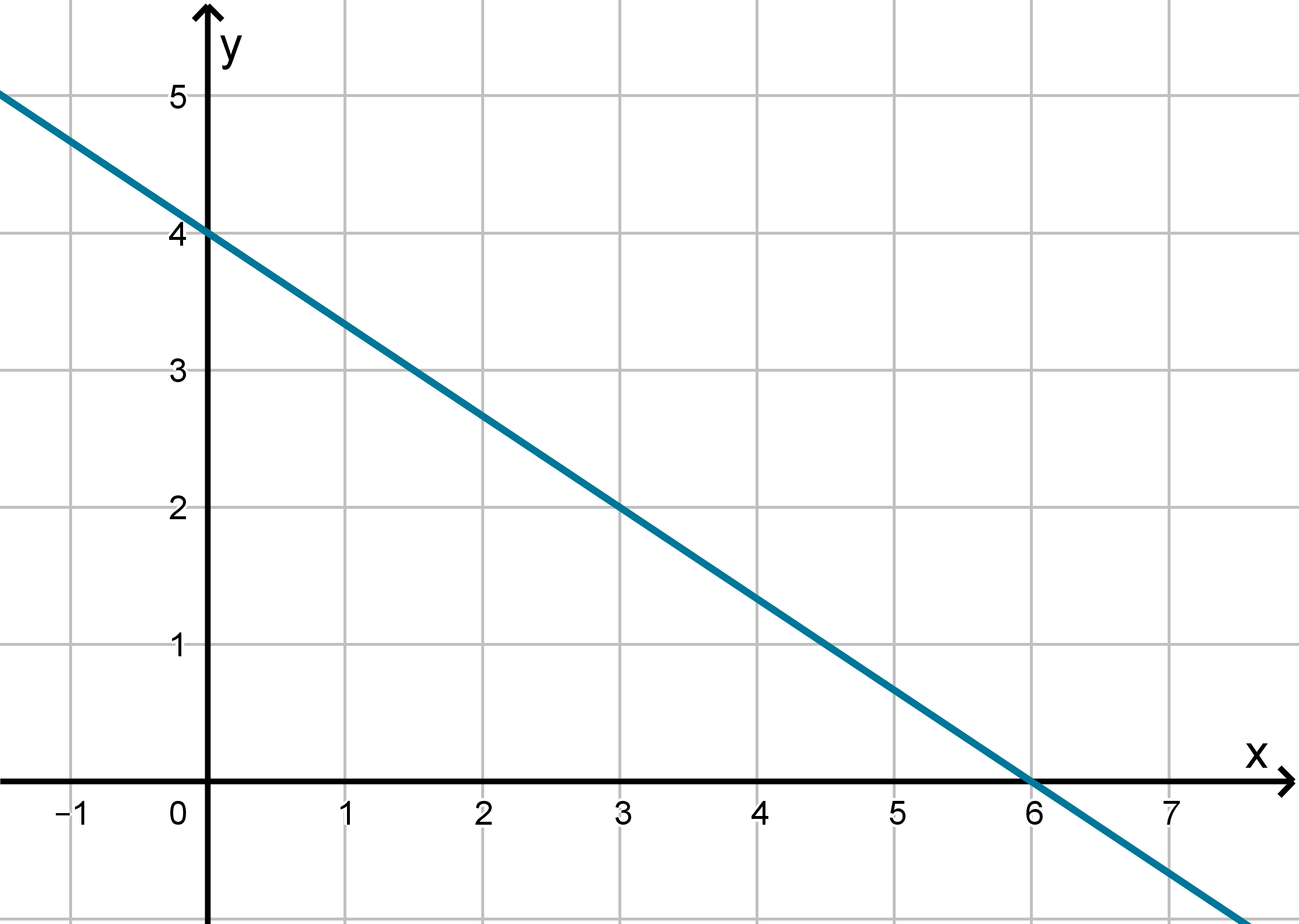
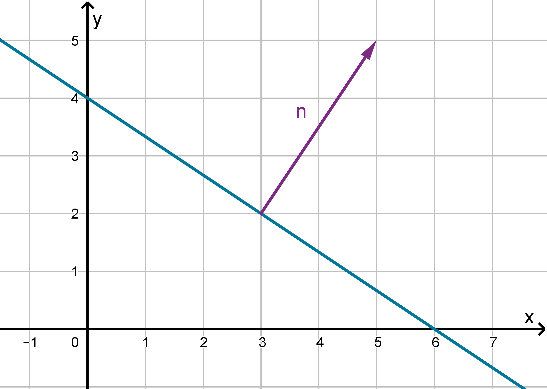
Question 5.3.1
What is a Normal Vector to a Plane?
In algebra, you learned the normal equation of a line: e.g.
2x + 3y − 12 = 0. Why is it called this?
373
Question 5.3.1
What is a Normal Vector to a Plane?
In algebra, you learned the normal equation of a line: e.g.
2x + 3y − 12 = 0. Why is it called this?
373
Question 5.3.1
What is a Normal Vector to a Plane?
A normal vector to a plane is orthogonal to every vector in the plane.
Theorem
In three-dimensional space, every plane has normal vectors. They are all
parallel to each other.
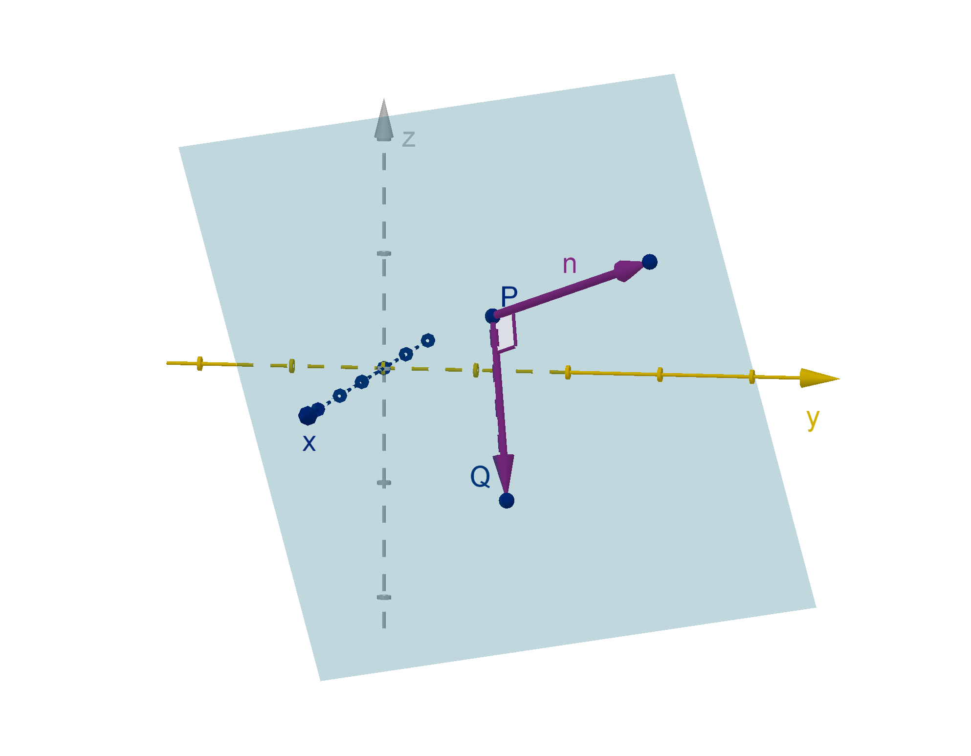
Figure: A plane, its normal vector
n, and a vector
−→
PQ in the plane
374
Question 5.3.1
What is a Normal Vector to a Plane?
Theorem
If
r
0
= ⟨x
0
, y
0
, z
0
⟩ describes an known point on a plane, and
n = ⟨a, b, c⟩
is a normal vector. Then the normal equation of the plane is
(
r −
r
0
) ·
n = 0
or
a(x − x
0
) + b(y − y
0
) + c(z − z
0
) = 0
img/normalequation.png
Notice that since x
0
, y
0
and z
0
are constants, we can distribute and
collect them into a single term: d.
ax + by + cz − ax
0
− by
0
− cz
0
= 0
ax + by + cz + d = 0
375
Question 5.3.1
What is a Normal Vector to a Plane?
This reasoning works in any dimension to define a set of points whose
displacement from a known point is orthogonal to some normal vector.
Example
a(x − x
0
) + b(y − y
0
) = 0 defines a line.
a(x − x
0
) + b(y − y
0
) + c(z − z
0
) = 0 defines a plane.
a
1
(x
1
− c
1
) + a
2
(x
2
− c
2
) + ··· + a
n
(x
n
− c
n
) = 0 defines a
hyperplane.
376
Example 5.3.2
Computing a Normal Vector
Find the normal equation of the plane with intercepts (4, 0, 0), (0, 3, 0)
and (0, 0, 8). Compute a normal vector.
377
Synthesis 5.3.3
Using the Normal Vector to Compute Distance
Consider the line 2x + 3y − 12 = 0.
This is the line with normal vector
n = ⟨2, 3⟩ and known point P = (3, 2).
378
Synthesis 5.3.3
Using the Normal Vector to Compute Distance
Example
Let P
1
= (7, 2) and P
2
= (4, 0).
1 Draw the vectors
−−→
PP
1
and
−−→
PP
2
.
2 If you didn’t have a picture, how could you use the values of
n ·
−−→
PP
1
and
n ·
−−→
PP
2
to determine which side of the line P
1
and P
2
lie on?
379
Synthesis 5.3.3
Using the Normal Vector to Compute Distance
Theorem
Given a line, plane, or hyperplane with normal equation L(x
1
, . . . , x
k
) = 0
and corresponding normal vector
n, the signed distance from the
hyperplane to the point Q = (q
1
, . . . , q
k
) is
L(q
1
, . . . , q
k
)
n
.
380
Example 5.3.4
The Distance from a Plane
Compute the geometric distance from the origin to the plane
6x + 8y + 3z − 24 = 0.
381
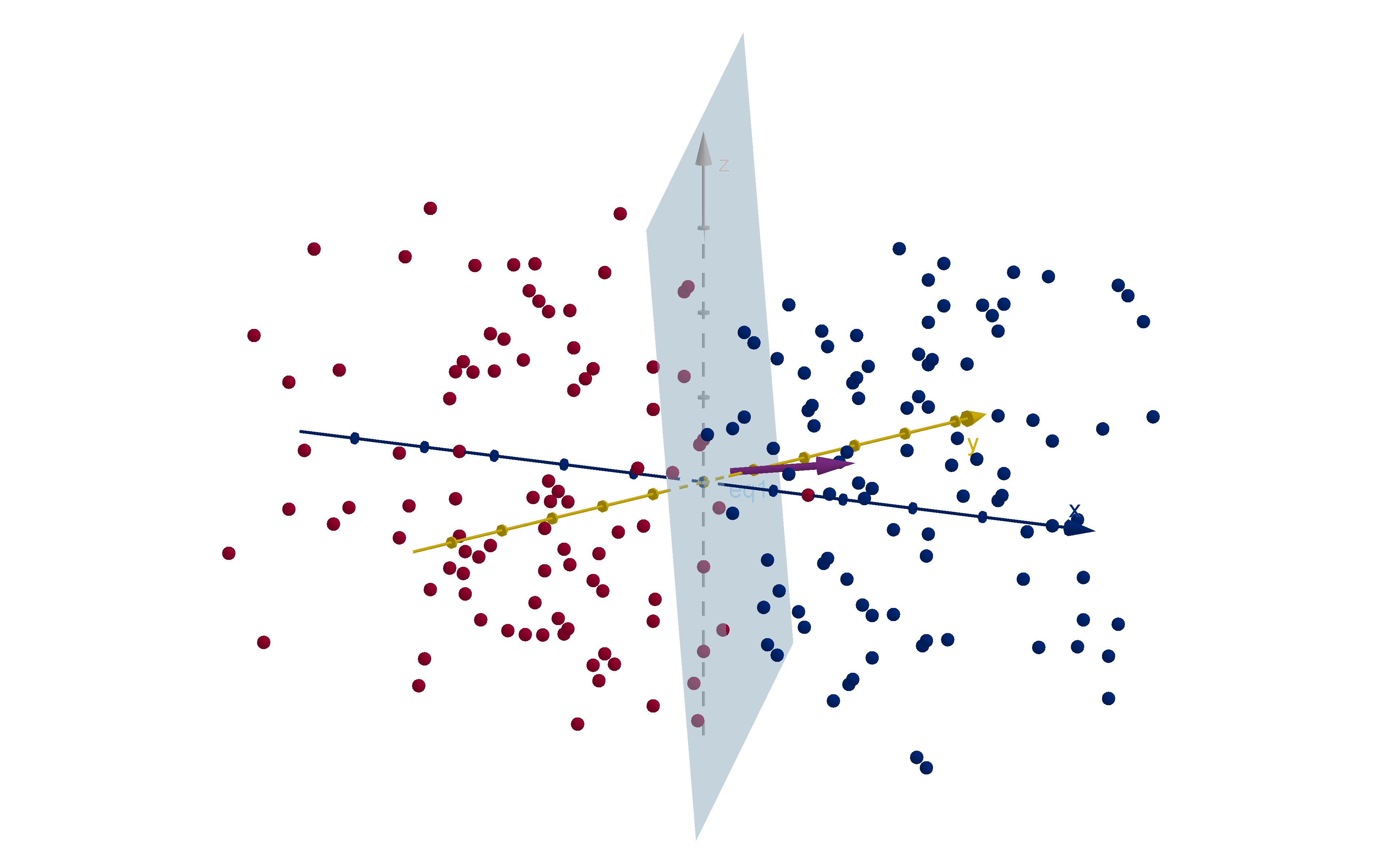
Application 5.3.5
Support Vector Machines
One type of machine learning involves training a computer to distinguish
between two states. For example, a computer might be trained to
distinguish between a cancerous tumor and a benign one.
To do this the computer is given a large set of cases. Each case is
measured by numerical data, such as:
The size of the tumor
The location of the tumor
The age of the patient
Results of blood tests
The brightness of each pixel in a CT scan or MRI
Each data type is a dimension, and each case is a point in a (probably
very high) dimensional space.
382
Application 5.3.5
Support Vector Machines
383
Section 5.3
Summary Questions
Q1 What information do you need in order to write the normal equation
of a plane?
Q2 How are the normal vectors of a plane related to each other?
Q3 What is the significance of the coefficients in the normal equation of
a plane?
Q4 How do we compute the signed distance from a point to a plane?
384
Section 5.3
Q14
Suppose we know the planes 12x + 18y + 6z − 15 = 0 and
ax + by + 4z + d = 0 are parallel. What can you say about the values of
a, b and d?
385
Section 5.3
Q30
Two planes are perpendicular if their normal vectors are orthogonal.
a Are 4x − 7y + z − 3 = 0 and 5x + y + 13z + 25 = 0 perpendicular?
b If two planes are perpendicular, is every vector in the first plane
orthogonal to every vector in the second plane?
386
Section 5.4
The Gradient Vector
Goals:
1 Calculate the gradient vector of a function.
2 Relate the gradient vector to the shape of a graph and its level
curves.
3 Compute directional derivatives.
Question 5.4.1
How Do We Compute Rates of Change in Another Direction?
The partial derivatives of f (x, y) give the instantaneous rate of change in
the x and y directions. This is realized geometrically as the slope of the
tangent line. What if we want to travel in a different direction?
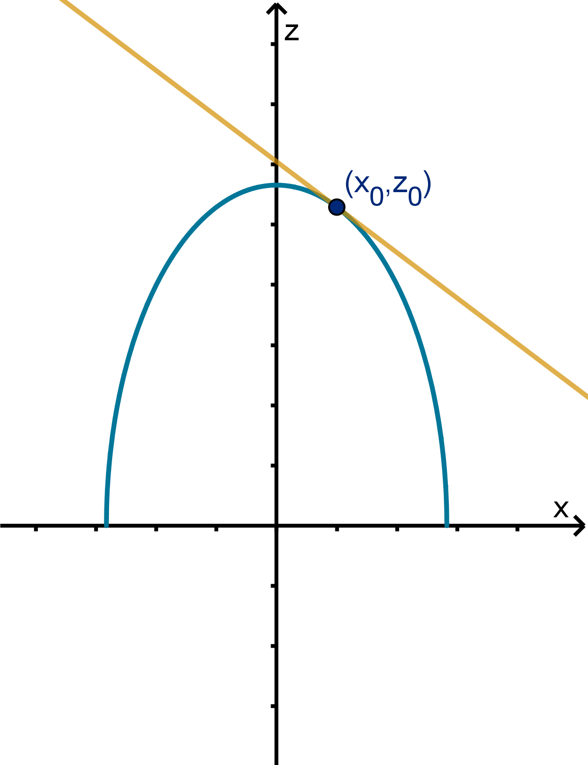
Figure: The tangent line to z = f (x, y ) in the x direction
388
Question 5.4.1
How Do We Compute Rates of Change in Another Direction?
Definition
Let f (x, y) be a function and
u be a unit vector in R
2
. The directional
derivative, denoted D
u
f , is the instantaneous rate of change of f as we
move in the
u direction. This is also the slope of the tangent line to
y = f (x, y ) in the direction of
u.
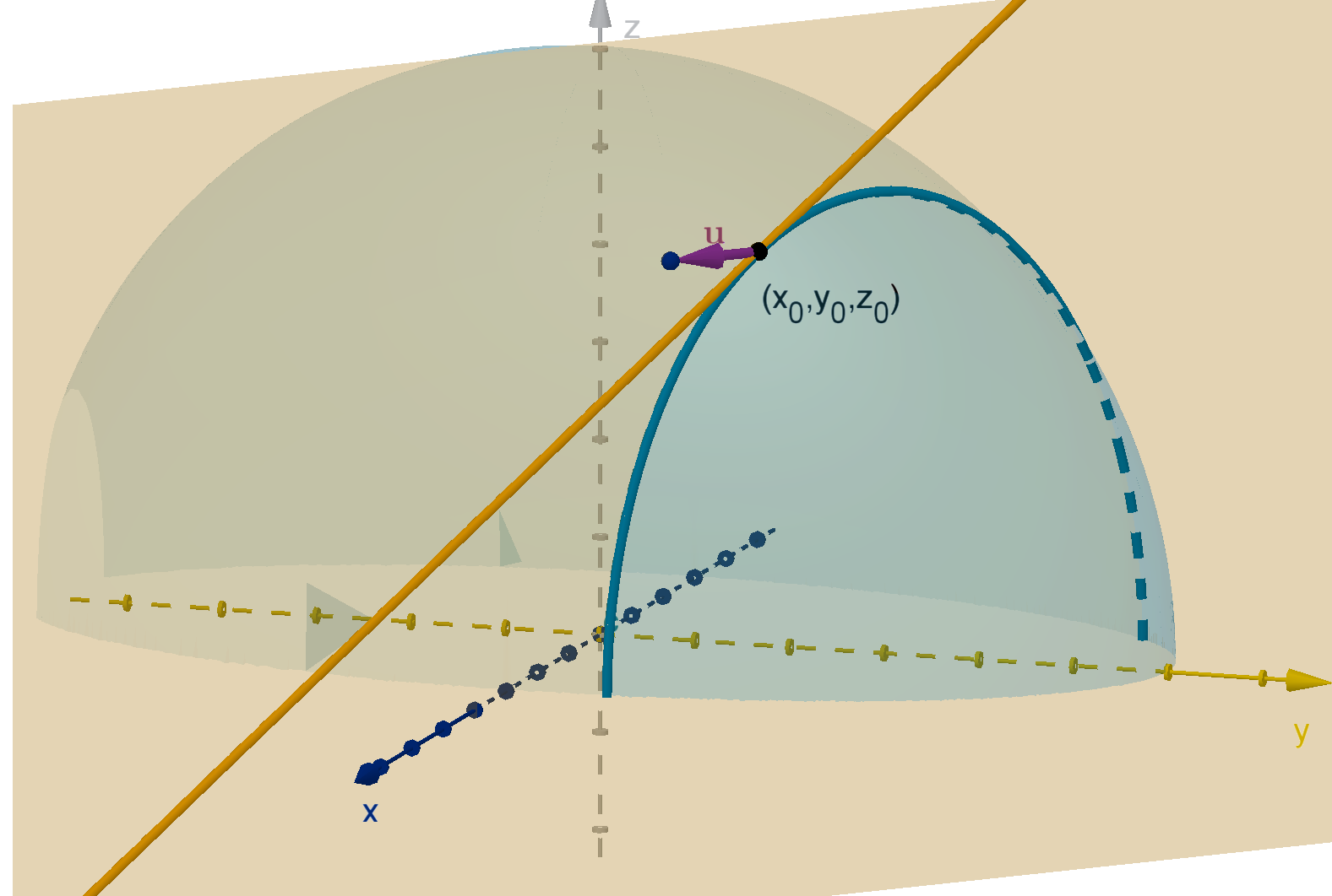
Figure: The tangent line to f (x, y) in the direction of
u
389
Question 5.4.1
How Do We Compute Rates of Change in Another Direction?
Recall that we compute D
x
f by comparing the values of f at (x, y) to
the value at (x + h, y ), a displacement of h in the x-direction.
D
x
f (x, y) = lim
h→0
f (x + h, y) −f (x, y )
h
To compute D
u
f for
u = a
i + b
j, we compare the value of f at (x, y ) to
the value at (x + ta, y + tb), a displacement of t in the
u-direction.
Limit Formula
D
u
f (x, y) = lim
t→0
f (x + ta, y + tb) −f (x, y )
t
390
Question 5.4.1
How Do We Compute Rates of Change in Another Direction?
Questions:
1 What direction produces the greatest directional derivative? The
smallest?
2 How are these directions related to the geometry (specifically the
level curves) of the graph?
3 How these directions related to the partial derivatives?
391
Question 5.4.1
How Do We Compute Rates of Change in Another Direction?
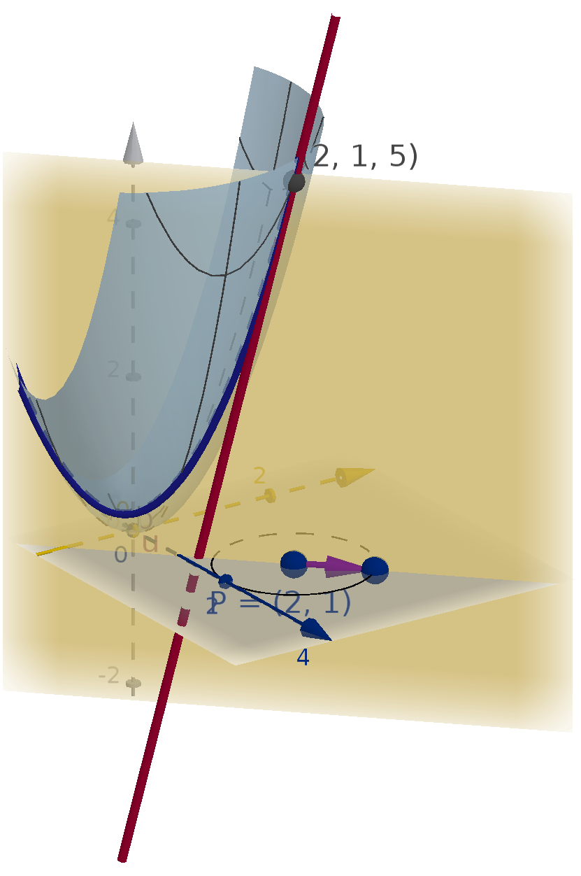
Figure: A cross section of z = f (x, y ) and a tangent line in the direction of
u
392
Question 5.4.2
What Is the Gradient Vector?
Definition
The gradient vector of f at (x, y ) is
∇f (x, y) = ⟨f
x
(x, y ), f
y
(x, y )⟩
Remarks:
1 The gradient vector is a function of (x, y ). Different points have
different gradients.
2
u
max
, which maximizes D
u
f , points in the same direction as ∇f .
3
u
0
, which is tangent to the level curves, is orthogonal to ∇f .
393
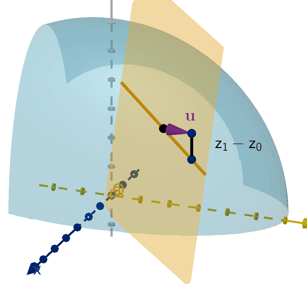
Question 5.4.3
How Do We Compute a Directional Derivative?
The tangent lines live in the tangent plane. We can compute their slope
by rise over run.
Let
u be a unit vector from (x
0
, y
0
) to (x
1
, y
1
). Let the associated z
values in the tangent plane be z
0
and z
1
respectively.
D
u
f (x
0
, y
0
) =
rise
run
=
z
1
− z
0
|
u|
=f
x
(x
0
, y
0
)(x
1
− x
0
) + f
y
(x
0
, y
0
)(y
1
− y
0
)
=∇f (x
0
, y
0
) ·
u.
394
Question 5.4.3
How Do We Compute a Directional Derivative?
Functions of More Variables
We can also define directional derivatives of higher variable functions
with analogous results.
f (x
1
, . . . , x
n
) is a differentiable function.
u is a unit vector in R
n
.
D
u
f denotes the directional derivative in the direction of
u.
∇f = ⟨f
x
1
, . . . , f
x
n
⟩ is an n-dimensional vector function on R
n
.
D
u
f = ∇f ·
u
395
Synthesis 5.4.4
Directional Derivative and the Cosine Formula
Now that we have a formula for directional derivatives, we can verify our
observations from earlier. Suppose f (x, y ) is a differentiable function and
we can choose any unit vector
u.
a Write D
u
f (x, y) in terms of the length of a vector and an angle.
b In what direction
u will f increase fastest?
c What will be the value of D
u
f (x, y) in that direction?
d In what direction
u will D
u
f (x, y) = 0?
396
Synthesis 5.4.4
Directional Derivative and the Cosine Formula
Figure: The angle between the gradient of f and a unit vector
Main Ideas
The cosine formula for the dot product lets us relate the directional
derivative to an angle.
f increases fastest in the direction of ∇f (x, y ).
D
u
f (x, y) = 0 when ∇f (x, y) and
u are orthogonal.
397
Example 5.4.5
A Directional Derivative
Let f (x, y) =
p
9 −x
2
− y
2
and let
u = ⟨0.6, −0.8⟩.
a What are the level curves of f ?
b What direction does ∇f (1, 2) point?
c Without calculating, is D
u
f (1, 2) positive or negative?
d Calculate ∇f (1, 2) and D
u
f (1, 2).
398
Example 5.4.6
Drawing the Gradient
Let h(x, y ) give the altitude at longitude x and latitude y. Assuming h is
differentiable, draw the direction of ∇h(x, y) at each of the points
labeled below. Which gradient is the longest?
A
B
C
Figure: A topographical map
399
Application 5.4.7
Edge Detection
The length of the gradient of a brightness function detects the edges in a
picture, where the brightness is changing quickly.
∂B
∂x
(336, 785) ≈
185−187
1
∂B
∂y
(336, 785) ≈
179−187
1
∇B(336, 785) ≈ (−2, −8)
∂B
∂x
(340, 784) ≈
97−139
1
∂B
∂y
(340, 784) ≈
72−139
1
∇B(340, 784) ≈ (−42, −67)
∇B
∇B
Figure: A long gradient vector indicates a swift change in brightness. Its
direction suggests the shape of the edges.
400
Application 5.4.8
Tangent Planes to a Level Surface
Use a gradient vector to find the equation of the tangent plane to the
graph x
2
+ y
2
+ z
2
= 14 at the point (2, 1, −3).
401
Application 5.4.8
Tangent Planes to a Level Surface
Main Idea
The graph of an implicit equation can be written as a level set of a
function. The gradient of that function is a normal vector to the level set
and also to its tangent line/plane/hyperplane.
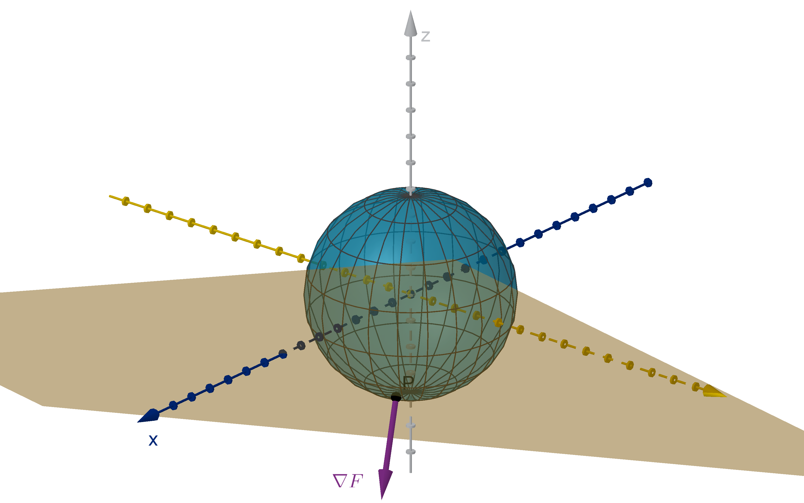
Figure: The level surface x
2
+ y
2
+ z
2
= 14, its tangent plane and ∇F .
402
Section 5.4
Summary Questions
Q1 What does the direction of the gradient vector tell you?
Q2 What does the directional derivative mean geometrically?
Q3 How do you compute a directional derivative?
Q4 How is the gradient vector related to a level set?
403
Section 5.4
Q12
Suppose the linearization of f (x, y ) at (−3, 9) has the equation
L(x, y ) = 4 + 2(x + 3) −
1
3
(y − 9).
What is the slope of L from (−3, 9) to (5, 3)?
404
Section 5.4
Q14
If D
u
f (x, y) < 0, what can you say about the directions of ∇f (x, y ) and
u?
405
Section 5.4
Q16
Explain why it makes sense that if D
u
f (a, b, c) = 0, then
u is tangent to
the level surface of f through (a, b, c).
406
Section 5.4
Q26
The brightness function on the Mona Lisa image ranges from 0 to 255. If
we use adjacent points to apporixmate the gradient as in the example,
what is the longest gradient vector we could theoretically produce?
407
Section 5.4
Q28
Let P be a point on the circle x
2
+ y
2
= r
2
. Show that the position
vector of P is normal to the circle at P.
408
Section 5.4
Q36
Suppose that f (x, y , z) is a differentiable function, and f (3, 5, −2) = 13.
Suppose further that the vectors ⟨3, 1, 0⟩ and ⟨0, 2, 5⟩ both lie in the
tangent plane to the surface f (x, y, z) = 13 at (3, 5, −2). If the
maximum value of D
u
f (3, 5, −2) is 20, find all possible values of
∇f (3, 5, −2).
409
Section 5.5
The Chain Rule
Goals:
1 Use the chain rule to compute derivatives of compositions of
functions.
2 Perform implicit differentiation using the chain rule.
Section 5.5 The Chain Rule
Motivational Example
Suppose Jinteki Corporation makes widgets which is sells for $100 each.
It commands a small enough portion of the market that its production
level does not affect the demand (price) for its products. If W is the
number of widgets produced and C is their operating cost, Jinteki’s
profit is modeled by
P = 100W − C
The partial derivative
∂P
∂W
= 100 does not correctly calculate the effect of
increasing production on profit. How can we calculate this correctly?
411
Question 5.5.1
How Can We Visualize a Composition with a Multivariable Function?
We can visualize a parametric equation as particle traveling through
space.
The variable t represents time.
x(t) and y(t) represent the coordinates of the position at time t.
The vector ⟨x
′
(t), y
′
(t)⟩ represents velocity. It points in the
direction of travel.
412
Question 5.5.1
How Can We Visualize a Composition with a Multivariable Function?
Figure: A particle whose position is defined by x(t) and y (t), the path it follows
and its velocity vector
413
Question 5.5.1
How Can We Visualize a Composition with a Multivariable Function?
Given a function f (x, y ) where x = x(t) and y = y (t), we can ask how f
changes as t changes. We can visualize this change by drawing the graph
z = f (x, y) over the path given by the parametric equations x(t) and
y(t).
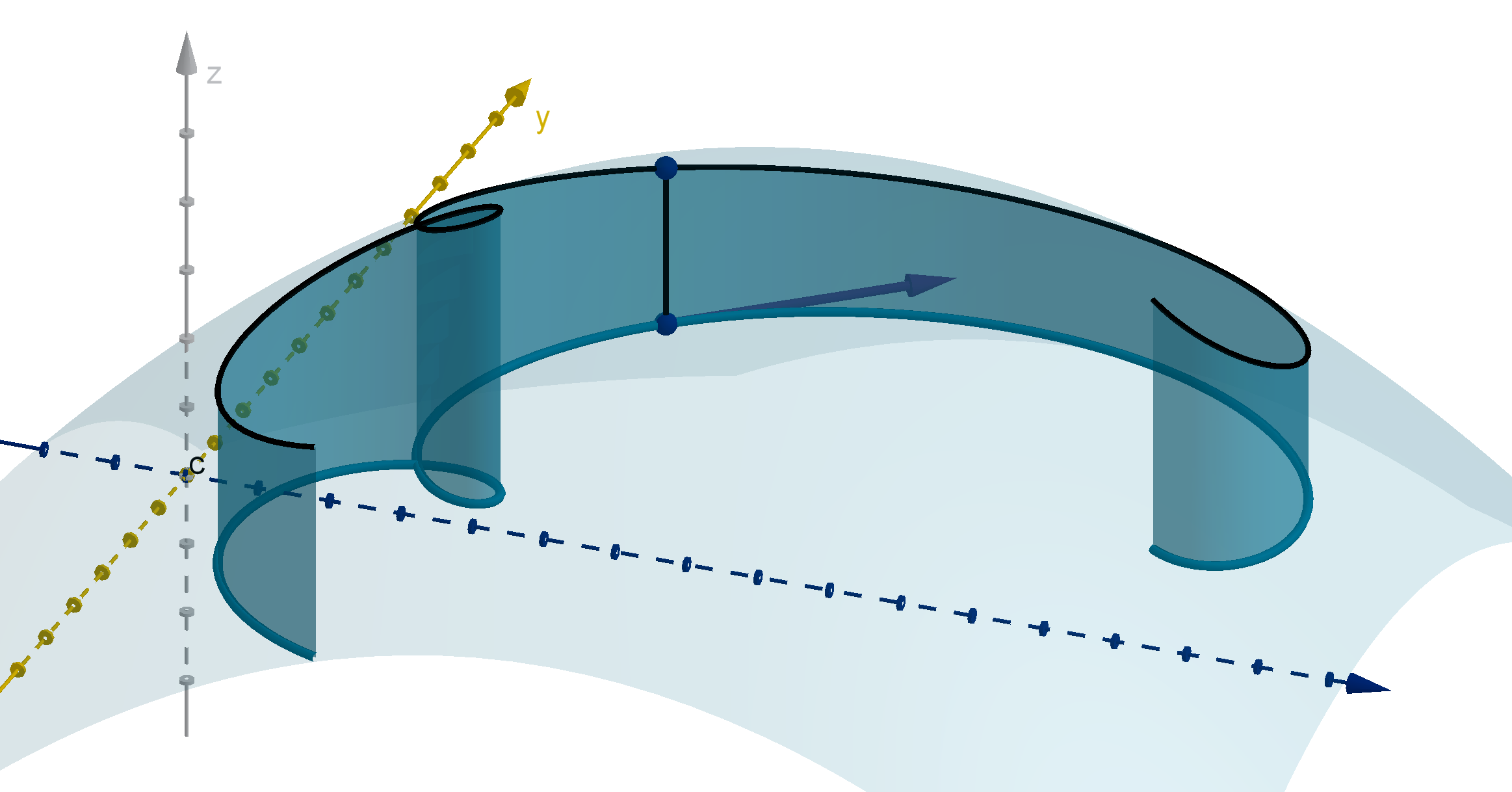
Figure: The composition f (x(t), y(t)), represented by the height of z = f (x , y)
over the path (x(t), y(t))
414
Question 5.5.2
How Do We Compute the Derivative of a Composition of Functions?
Theorem (The Chain Rule)
Consider a differentiable function f (x, y). If we define x = x(t) and
y = y (t), both differential functions, we have
df
dt
=
∂f
∂x
dx
dt
+
∂f
∂y
dy
dt
or
df
dt
= ∇f (x, y) · ⟨x
′
(t), y
′
(t)⟩
415
Question 5.5.2
How Do We Compute the Derivative of a Composition of Functions?
Remarks
f (x(t), y(t)) is a function (only) of t. Because of this,
df
dt
is an
ordinary derivative, not a partial derivative.
df
dt
is not the slope of the composition graph.
slope =
rise in z
run in xy-plane
df
dt
=
rise in z
change in t
The chain rule is easy to remember because of its similarity to the
differential:
dz =
∂z
∂x
dx +
∂z
∂y
dy.
The proof is more complicated than just sticking a dt under each
term.
416
Example 5.5.3
Using the Chain Rule
If P = R − C and we have R = 100w and C = 3000 + 70w − 0.1w
2
,
calculate
dP
dw
.
417
Question 5.5.4
What If We Have More Variables?
The chain rule works just as well if x and y are functions of more than
one variable. In this case it computes partial derivatives.
Theorem
If f (x, y), x(s, t) and y (s, t), are all differentiable, then
∂f
∂s
=
∂z
∂x
∂x
∂s
+
∂z
∂y
∂y
∂s
or
∂f
∂s
= ∇f (x, y) ·
∂x
∂s
,
∂y
∂s
418
Question 5.5.4
What If We Have More Variables?
We can also modify it for functions of more than two variables.
Theorem
Given f (x, y, z), x(t), y(t) and z(t), all differentiable, we have
df
dt
=
∂f
∂x
dx
dt
+
∂f
∂y
dy
dt
+
∂f
∂z
dz
dt
or
df
dt
= ∇f (x, y, z) ·⟨x
′
(t), y
′
(t), z
′
(t)⟩
419
Example 5.5.5
A Composition with More Variables
Recall that for an ideal gas P(n, T , V ) =
nRT
V
. R is a constant. n is the
number of molecules of gas. T is the temperature in Celsius. V is the
volume in meters. Suppose we want to understand the rate at which the
pressure changes as an air-tight glass container of gas is heated.
a Apply the chain rule to get an expression for
dP
dT
.
b What is
dn
dT
?
c What is
dT
dT
?
d Suppose that
dV
dT
= (5.9 ×10
−6
)V . Calculate and simplify the
expression you got for
dP
dT
.
420
Example 5.5.5
A Composition with More Variables
Recall that for an ideal gas P(n, T , V ) =
nRT
V
. R is a constant. n is the
number of molecules of gas. T is the temperature in Celsius. V is the
volume in meters. Suppose we want to understand the rate at which the
pressure changes as an air-tight glass container of gas is heated.
a Apply the chain rule to get an expression for
dP
dT
.
420
Example 5.5.5
A Composition with More Variables
Recall that for an ideal gas P(n, T , V ) =
nRT
V
. R is a constant. n is the
number of molecules of gas. T is the temperature in Celsius. V is the
volume in meters. Suppose we want to understand the rate at which the
pressure changes as an air-tight glass container of gas is heated.
b What is
dn
dT
?
420
Example 5.5.5
A Composition with More Variables
Recall that for an ideal gas P(n, T , V ) =
nRT
V
. R is a constant. n is the
number of molecules of gas. T is the temperature in Celsius. V is the
volume in meters. Suppose we want to understand the rate at which the
pressure changes as an air-tight glass container of gas is heated.
c What is
dT
dT
?
420
Example 5.5.5
A Composition with More Variables
Recall that for an ideal gas P(n, T , V ) =
nRT
V
. R is a constant. n is the
number of molecules of gas. T is the temperature in Celsius. V is the
volume in meters. Suppose we want to understand the rate at which the
pressure changes as an air-tight glass container of gas is heated.
d Suppose that
dV
dT
= (5.9 ×10
−6
)V . Calculate and simplify the
expression you got for
dP
dT
.
420
Example 5.5.6
A Composition with Limited Information
Suppose g (p, q, r ) = re
p
2
q
. Given that p, q, r are all differentiable
functions of x with the values in the following table, compute
dg
dx
when
x = 2.
x 0 1 2 3
p(x) 3 1 5 10
p
′
(x) −3 2 3 4
q(x) 6 2 −2 3
q
′
(x) −1 −5 2 3
r(x) 10 11 7 3
r
′
(x) 1 0 −1 −3
421
Application 5.5.7
Implicit Differentiation
Recall that an implicit equation on n variables is a level curve of a
n-variable function. Consider the graph x
3
+ y
2
− 4xy = 0. How can we
use this to calculate
dy
dx
at the point (3, 3)?
422
Application 5.5.7
Implicit Differentiation
Figure: The graph of F (x, y ) = x
3
+ y
2
− 4xy = 0, its tangent line at (3, 3),
and the gradient of F
Main Ideas
dy
dx
is the slope of the tangent line to F (x, y) = c.
The chain rule allows us to derive
dy
dx
= −
F
x
F
y
−
F
x
F
y
is the negative reciprocal of
F
y
F
x
, which is the slope of ∇F .
423
Application 5.5.8
Indirect Profit Functions
Suppose a firm chooses how much quantity q to produce, but their profit
Π(q, α) depends on some parameter α outside their control (maybe a tax
or a measure of regulatory burden). The firm, once it knows the value of
α, will choose the q that maximizes profit. How will their profit change
as α changes?
424
Application 5.5.8
Indirect Profit Functions
Figure: Two graphs of z = Π(q, α), one where q changes to be the optimal
choice for each α and one where q is fixed at q
0
, the optimal choice for α
0
425
Section 5.5
Summary Questions
Q1 How can we visualize f (x, y ), when x and y are functions of t?
Q2 Explain why
df
dt
cannot be interpreted as a slope of f over the
xy-plane.
Q3 What is the difference between
dz
dx
and
∂z
∂x
? How is the first one
computed?
Q4 How do you use the chain rule to differentiate implicit functions?
426
Section 5.5
Q12
Liam says “If f is a function of x and y and x and y are increasing, then
f is increasing.” We all know Liam is incorrect. How could we use the
chain rule to refute him?
427
Section 5.5
Q14
Let x = t
2
and y = sin t. Let f (x, y) = xy .
a Compute
df
dt
using the multivariable chain rule.
b Compute
df
dt
by substituting and using single-variable differentiation.
c What earlier rule of differentiation can we recover by applying the
chain rule to f (x, y) = xy ?
428
Section 5.5
Q26
Another principle in physics is the conservation of energy. Kenetic energy
is given by E =
1
2
mv
2
, where m is the mass and v is the linear speed of
the object. Suppose that we have a rock drifiting through space.
Suppose it impacts stationary rocks and the combined mass sticks
together (without releasing any energy as heat, light or sound). Thus the
mass of the total travelling object increases, while the total energy stays
the same. Derive an expression for how speed changes per unit of
increase in mass.
429
Section 5.5
Q27
Suppose that x is a function of t and that when t = 9, we have x = 7
and
dx
dt
= −3. Define f (x, t) =
√
x + t.
a Compute the partial derivate
∂f
∂t
(7, 9).
b Compute the total derivative
df
dt
(7, 9).
c In a few sentences, explain what these two quantities compute and
why they are different from each other.
430
Section 5.5
Q30
Suppose the position of a particle at time t is given by
x(t) = t
2
y(t) = 3 − t
z(t) =
√
t
At t = 4, how quickly is particle travelling away from the plane
x + 2y − 2z = 10?
431
Section 5.5
Q31
Here is a diagram of the level curves of h(x, y) for certain values of c.
a Is h
y
(2, 1) positive or negative? Explain in a sentence or two.
b Add a vector to the diagram that indicates the direction of greatest
increase of h at (−2, 0).
c Suppose x = 4 − 5t and y = 3t
2
. Determine, with the aid of a
relevant calculation, whether
dh
dt
is positive or negative at t = 1.
432
Section 5.6
Maximum and Minimum Values
Goals:
1 Find critical points of a function.
2 Test critical points to find local maximums and minimums.
3 Use the Extreme Value Theorem to find the global maximum and
global minimum of a function over a closed set.
Question 5.6.1
What Are Local Extremes?
The local extremes of a function are the local minimums and
maximums.
Definition
Given an n-variable function f (x
1
, x
2
, . . . , x
n
) we say that a point P in
n-space is
1 a local maximum if f (P) ≥ f (Q) for all Q in some neighborhood
around P.
2 a local minimum if f (P) ≤ f (Q) for all Q in some neighborhood
around P.
434
Question 5.6.2
Where Do Local Extremes Lie?
If f
x
(P) = 0, then we could travel in the x direction to increase or
decrease f . If f
x
(P) = 0, then we could travel in the y direction to
increase or decrease f . Thus at a local maximum or local minimum, the
tangent plane must be horizontal.
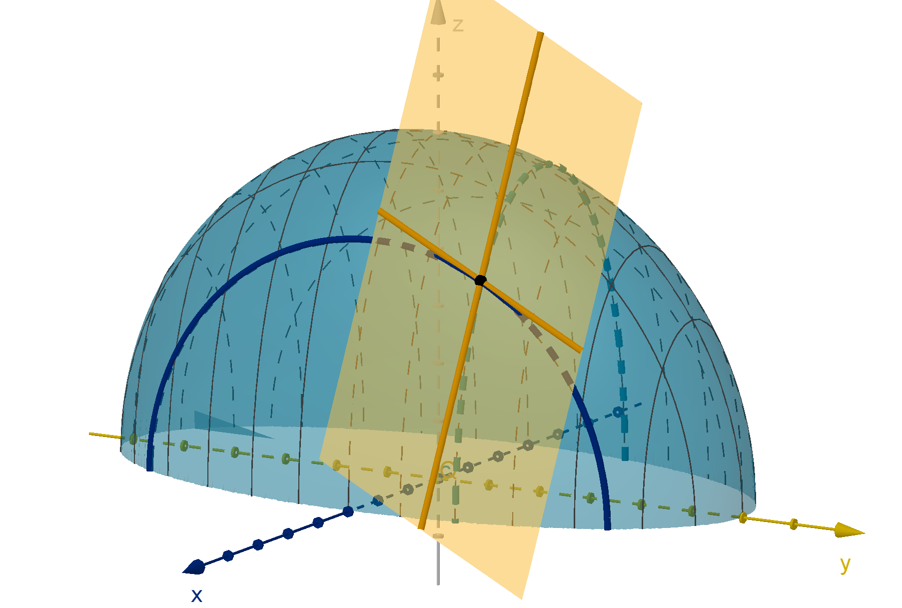
Figure: Tangent lines must have slope 0 at a local max.
435
Question 5.6.2
Where Do Local Extremes Lie?
Definition
We say P is a critical point of f if either
1 ∇f (P) =
0 or
2 ∇f (P) does not exist (because one of the partial derivatives does
not exist).
Theorem
The local maximums and minimums of a function can only occur at
critical points.
436
Example 5.6.3
Finding Critical Points
The function z = 2x
2
+ 4x + y
2
−6y + 13 has a minimum value. Find it.
437
Question 5.6.4
How Do We Identify Two-Variable Local Maximums and Minimums?
A critical point could be a local maximum. In this case f curves
downward in every direction.
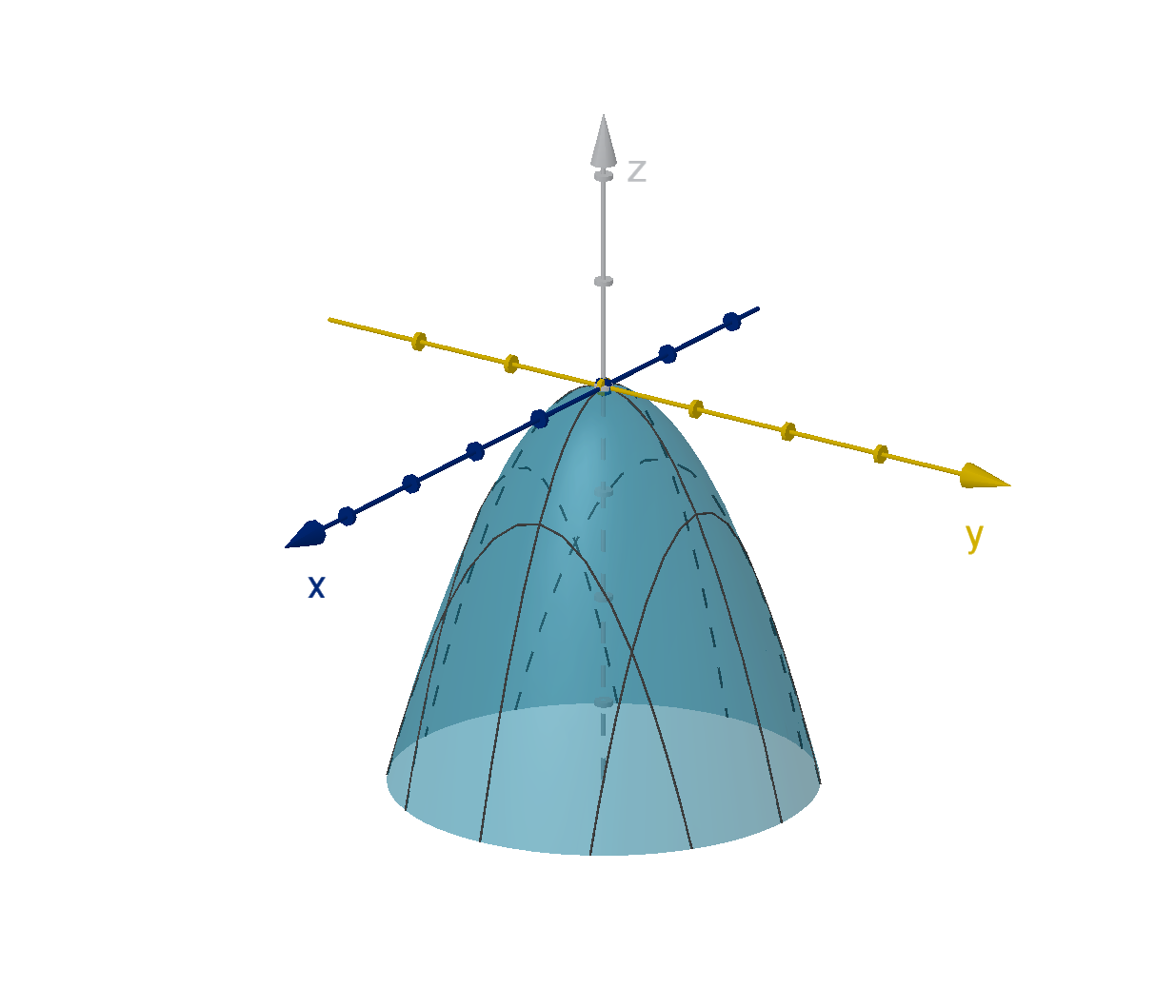
Figure: A local maximum at (0, 0)
438
Question 5.6.4
How Do We Identify Two-Variable Local Maximums and Minimums?
A critical point could be a local minimum. In this case f curves upward
in every direction.
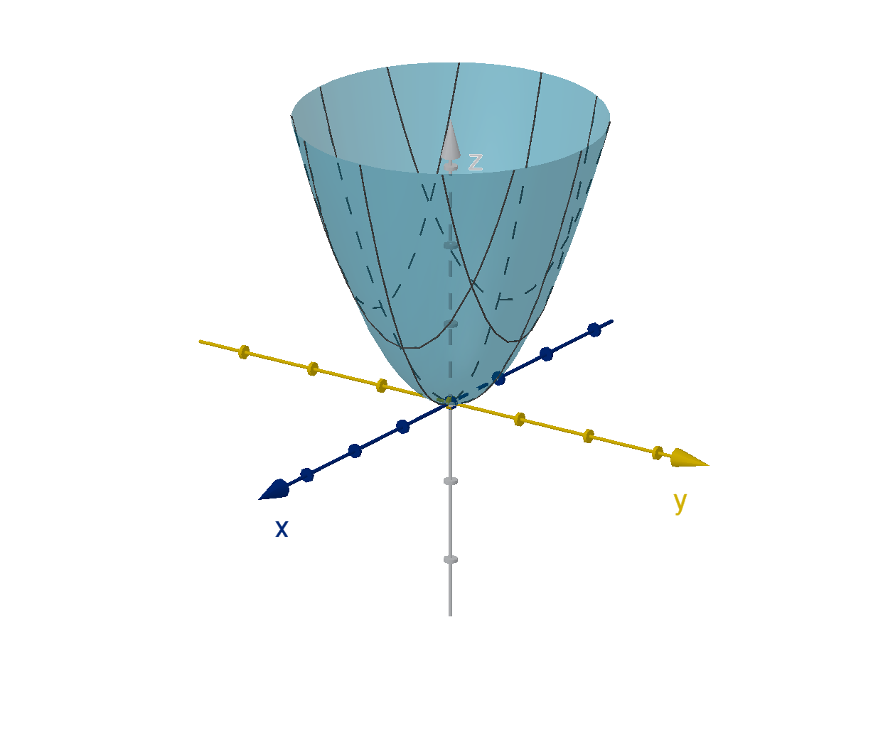
Figure: A local minimum at (0, 0)
439
Question 5.6.4
How Do We Identify Two-Variable Local Maximums and Minimums?
A critical point could be neither. f curves upward in some directions but
downward in others. This configuration is called a saddle point.
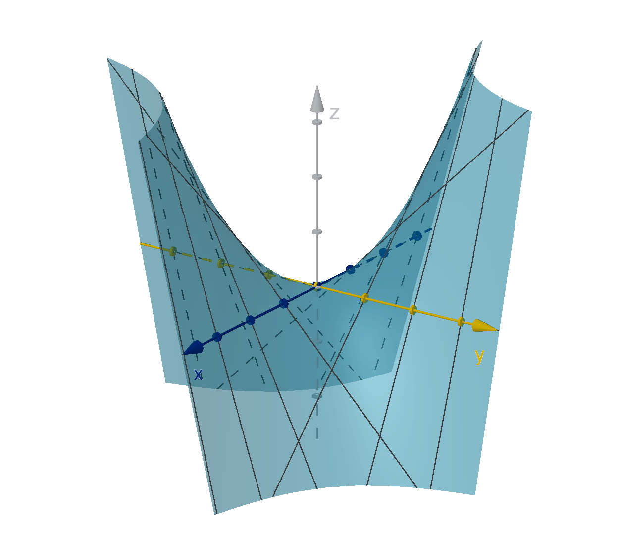
Figure: A saddle point at (0, 0)
440
Question 5.6.4
How Do We Identify Two-Variable Local Maximums and Minimums?
Theorem (The Second Derivatives Test)
Suppose f is differentiable at (P) and f
x
(P) = f
y
(P) = 0. Then we can
compute
D = f
xx
(P)f
yy
(P) −[f
xy
(P)]
2
1 If D > 0 and f
xx
(P) > 0 then P is a local minimum.
2 If D > 0 and f
xx
(P) < 0 then P is a local maximum.
3 If D < 0 then P is a saddle point.
Unfortunately, if D = 0, this test gives no information.
441
Question 5.6.4
How Do We Identify Two-Variable Local Maximums and Minimums?
Definition
The quantity D in the second derivatives test is actually the determinant
of a matrix called the Hessian of f .
f
xx
(P)f
yy
(P) −[f
xy
(P)]
2
= det
f
xx
(P) f
xy
(P)
f
yx
(P) f
yy
(P)
| {z }
Hf (P)
Hf follows a logical pattern and can be a useful mnemonic for the second
derivatives test.
442
Example 5.6.5
Classifying a Critical Point
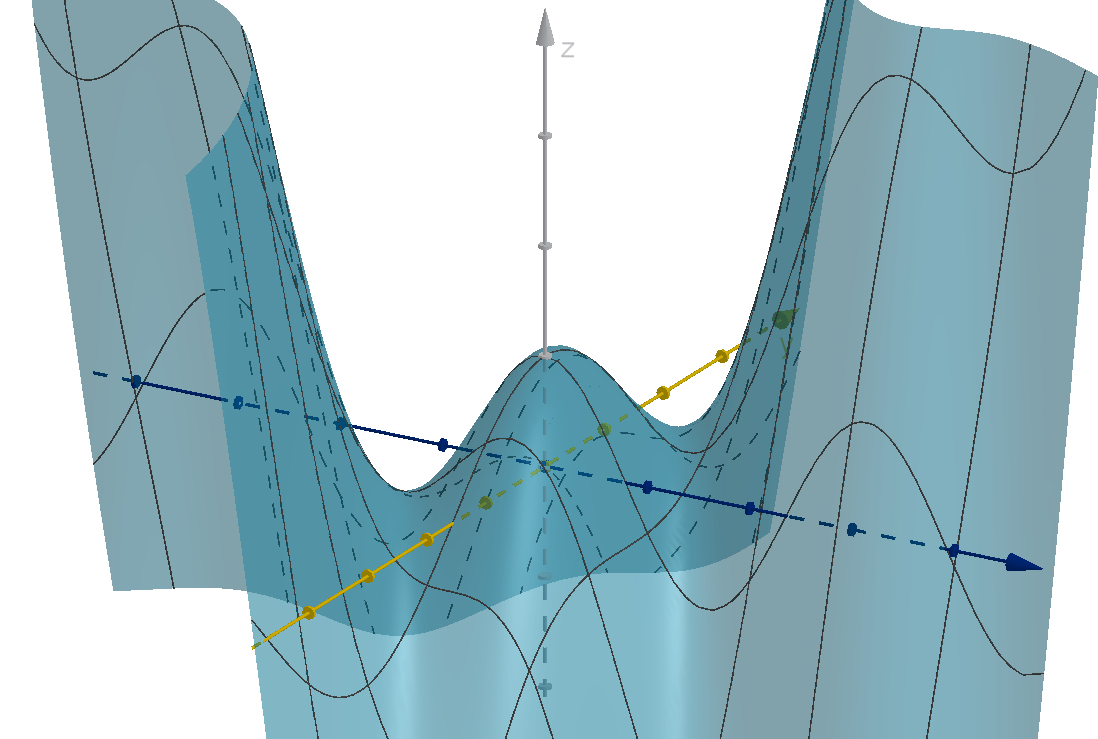
Figure: The graph z = cos(2x + y) + xy with a local maximum at (0, 0)
443
Question 5.6.6
How Do We Find Global Extremes?
Theorem (The Extreme Value Theorem)
A continuous function f on a closed and bounded domain D has a global
maximum and a global minimum somewhere in D.
Definition
Let D be a subset of n-space.
D is closed if it contains all of the points on its boundary.
D is bounded if there is some upper limit to how far its points get
from the origin (or any other fixed point). If there are points of D
arbitrarily far from the origin, then D is unbounded.
444
Question 5.6.6
How Do We Find Global Extremes?
For one-variable functions. The EVT requires that the domain be a union
of finite, closed intervals (and maybe finitely many isolated points).
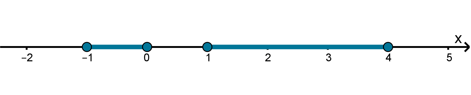
Figure: A union of finite, closed intervals
445
Question 5.6.6
How Do We Find Global Extremes?
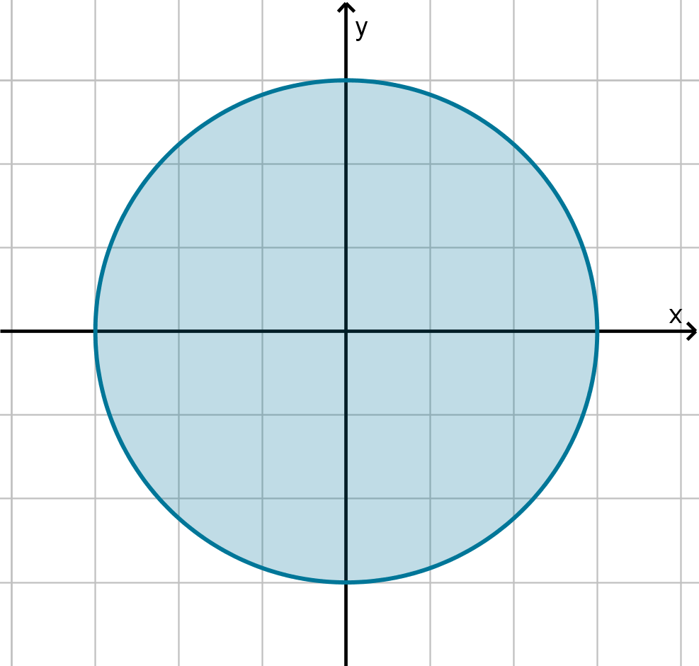
Figure: x
2
+ y
2
≤ 9 is closed.
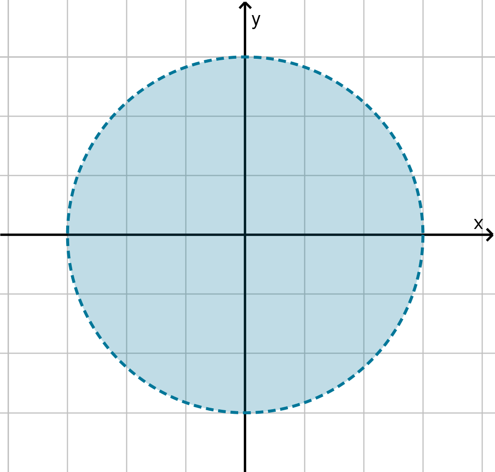
Figure: x
2
+ y
2
< 9 is not
closed.
446
Question 5.6.6
How Do We Find Global Extremes?
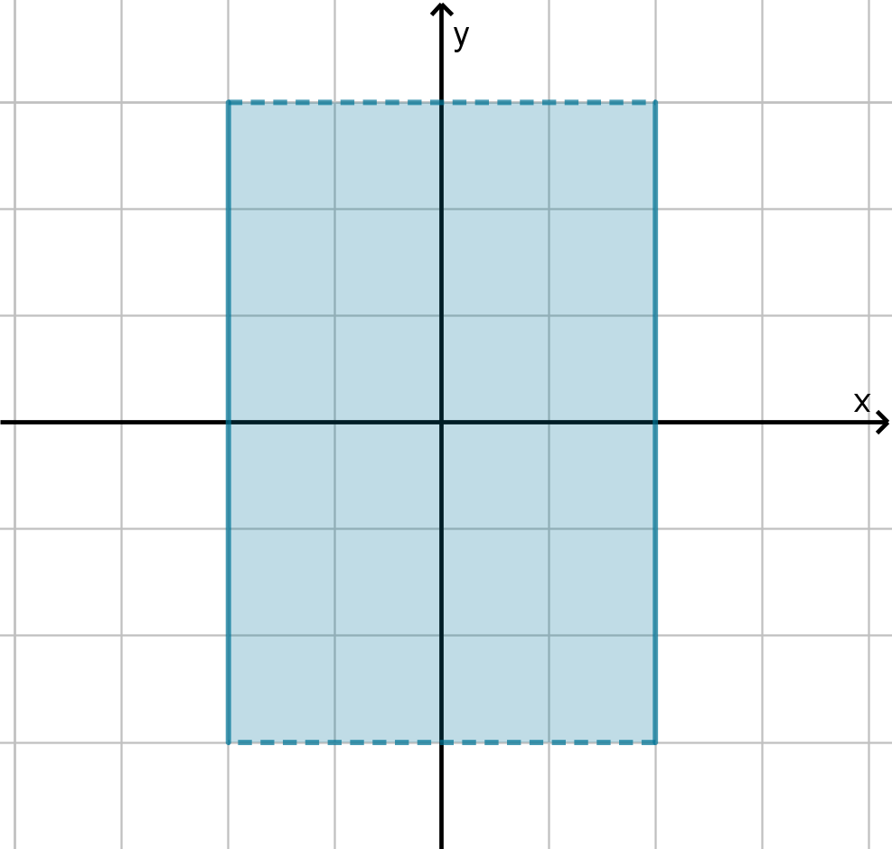
Figure: −2 ≤ x ≤ 2 and
−3 < y < 3 is not closed.
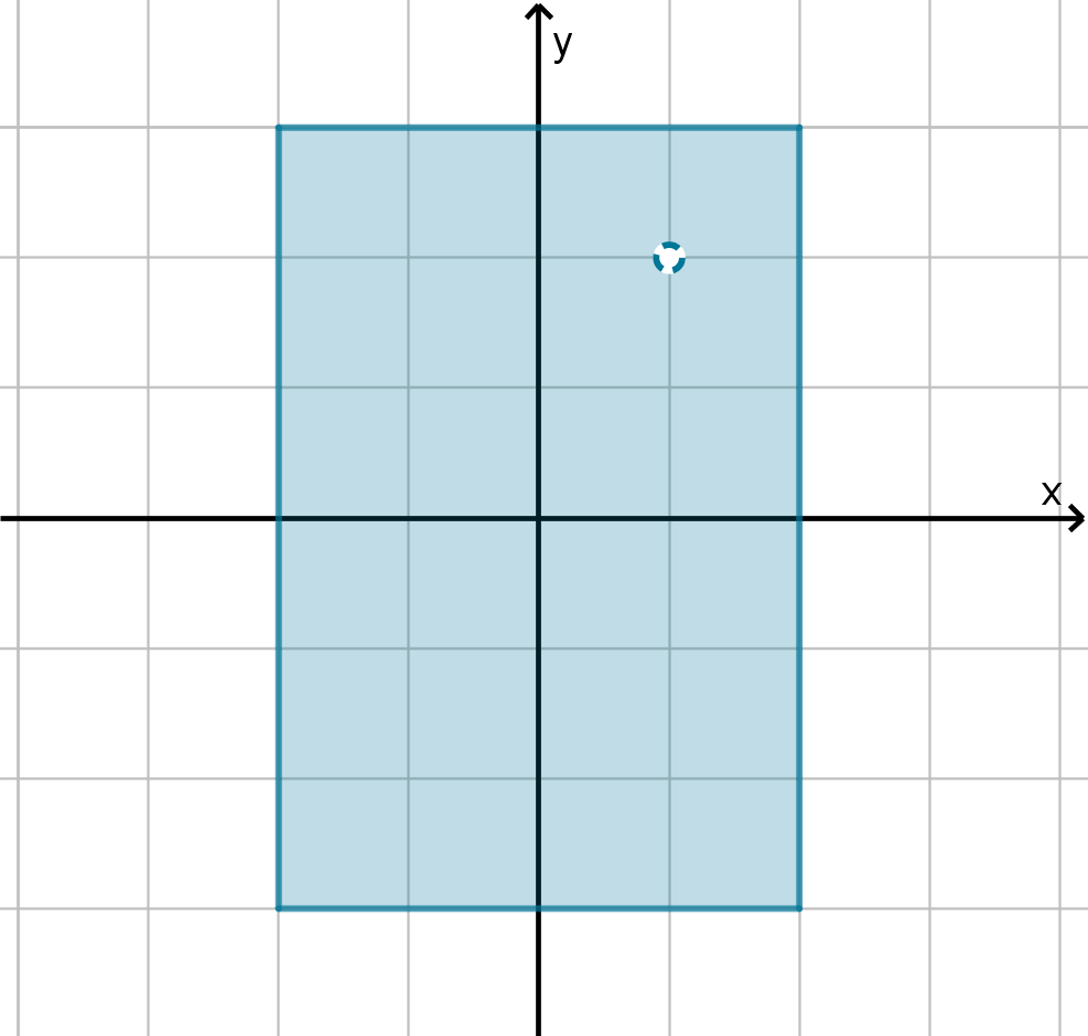
Figure: −2 ≤ x ≤ 2 and
−3 ≤ y ≤ 3 and (x, y) = (1, 2)
is not closed.
447
Question 5.6.6
How Do We Find Global Extremes?
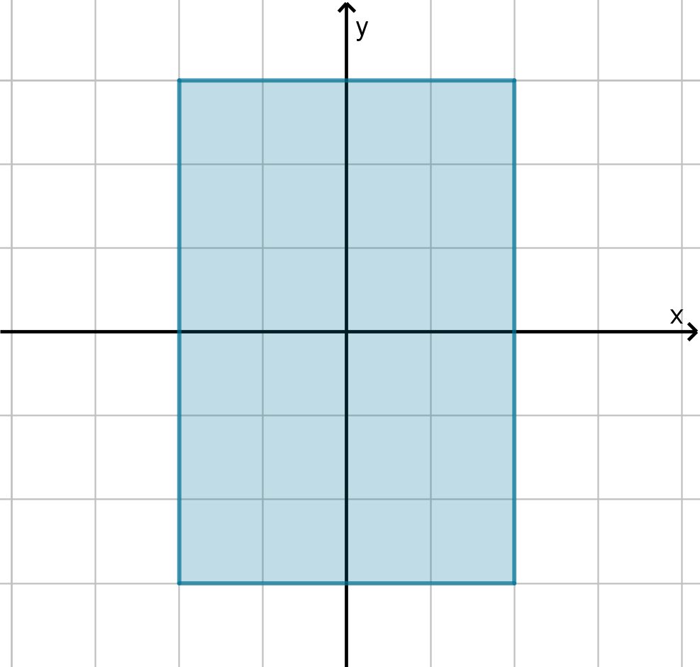
Figure: −2 ≤ x ≤ 2 and
−3 ≤ y ≤ 3 is bounded.
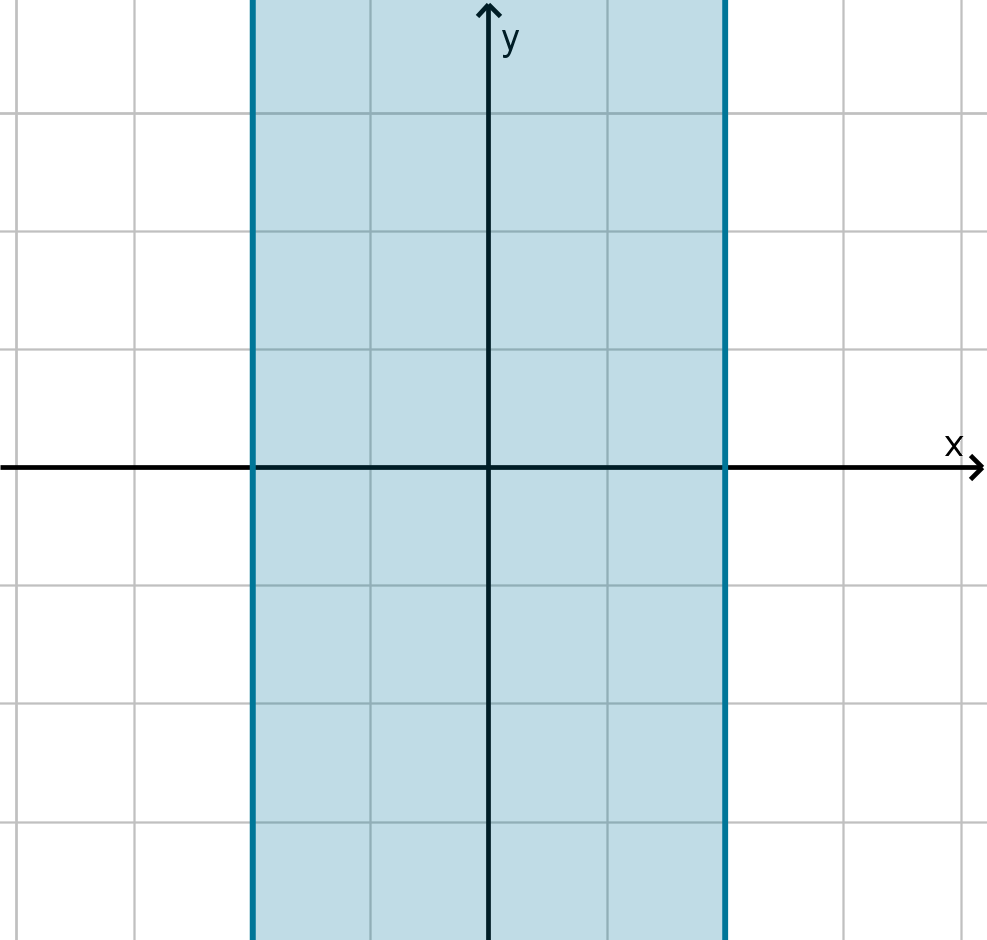
Figure: −2 ≤ x ≤ 2 is
unbounded.
448
Example 5.6.7
Finding a Global Maximum
Consider the function f (x, y) = x
2
+ 2y
2
− x
2
y on the domain
D = {(x, y) : x
2
+ y
2
≤ 16, x ≤ 0}
a Does f have a maximum value on D? How do we know?
b Find the critical points of f .
c Must one of the critical points be the maximum?
d Find the maximum of f .
449
Example 5.6.7
Finding a Global Maximum
Consider the function f (x, y) = x
2
+ 2y
2
− x
2
y on the domain
D = { (x, y )
|{z}
points in R
2
: x
2
+ y
2
≤ 16, x ≤ 0
| {z }
conditions
}
a Does f have a maximum value on D? How do we know?
449
Example 5.6.7
Finding a Global Maximum
Consider the function f (x, y) = x
2
+ 2y
2
− x
2
y on the domain
D = { (x, y )
|{z}
points in R
2
: x
2
+ y
2
≤ 16, x ≤ 0
| {z }
conditions
}
a Does f have a maximum value on D? How do we know?
449
Example 5.6.7
Finding a Global Maximum
Consider the function f (x, y) = x
2
+ 2y
2
− x
2
y on the domain
D = { (x, y )
|{z}
points in R
2
: x
2
+ y
2
≤ 16, x ≤ 0
| {z }
conditions
}
a Find the critical points of f .
449
Example 5.6.7
Finding a Global Maximum
Consider the function f (x, y) = x
2
+ 2y
2
− x
2
y on the domain
D = { (x, y )
|{z}
points in R
2
: x
2
+ y
2
≤ 16, x ≤ 0
| {z }
conditions
}
a Must one of the critical points be the maximum?
449
Example 5.6.7
Finding a Global Maximum
Consider the function f (x, y) = x
2
+ 2y
2
− x
2
y on the domain
D = { (x, y )
|{z}
points in R
2
: x
2
+ y
2
≤ 16, x ≤ 0
| {z }
conditions
}
a Find the maximum of f .
449
Example 5.6.7
Finding a Global Maximum
449
Example 5.6.7
Finding a Global Maximum
Main Ideas
If the Extreme Value Theorem applies, then all we need to do is find
the critical points and evaluate f at each. One is guaranteed to be
the maximum, and one is guaranteed to be the minimum.
∇f =
0 will detect critical points on the interior, but not on the
boundary.
We can rewrite the function on a boundary component using
substitution. Set the derivative equal to 0 to find critical points.
Derivatives will not detect maximums at the endpoints of a boundary
curve. These must be included in your set of critical points.
450
Section 5.6
Summary Questions
Q1 Where must the local maximums and minimums of a function
occur? Why does this make sense?
Q2 What does the second derivatives test tell us?
Q3 What hypotheses does the Extreme Value Theorem require? What
does it tell us?
Q4 Assuming a maximum and minimum exist, where must you look in a
domain to be sure you find them?
451
Section 5.6
Q6
Is a global maximum also a local maximum? Explain.
452
Section 5.6
Q12
Suppose f (x) is a function of x with critical points x = a and x = b.
Suppose g (y ) is a function of y with critical points y = c and y = d.
What are the critical points of h(x, y) = f (x) + g(y)?
453
Section 5.6
Q16
For what values of a does f (x, y) = x
2
+ y
2
+ axy have a local minimum
at the origin?
454
Section 5.6
Q32
Let f (x, y) be a differentiable function and let
D = {(x, y) : y ≥ x
2
− 4, x ≥ 0, y ≤ 5}.
a Sketch the domain D.
b Does the Extreme Value Theorem guarantee that f has an absolute
minimum on D? Explain.
c List all the places you would need to check in order to locate the
minimum.
455
Section 5.7
Lagrange Multipliers
Goals:
1 Find minimum and maximum values of a function subject to a
constraint.
2 If necessary, use Lagrange multipliers.
Question 5.7.1
What Is a Constraint?
Sometimes we aren’t interested in the maximum value of f (x, y ) over the
whole domain, we want to restrict to only those points that satisfy a
certain constraint equation.
The maximum on the constraint
is unlikely to be the same as the
unconstrained maximum (where
∇f = 0). Can we still use ∇f
to find the maximum on the
constraint?
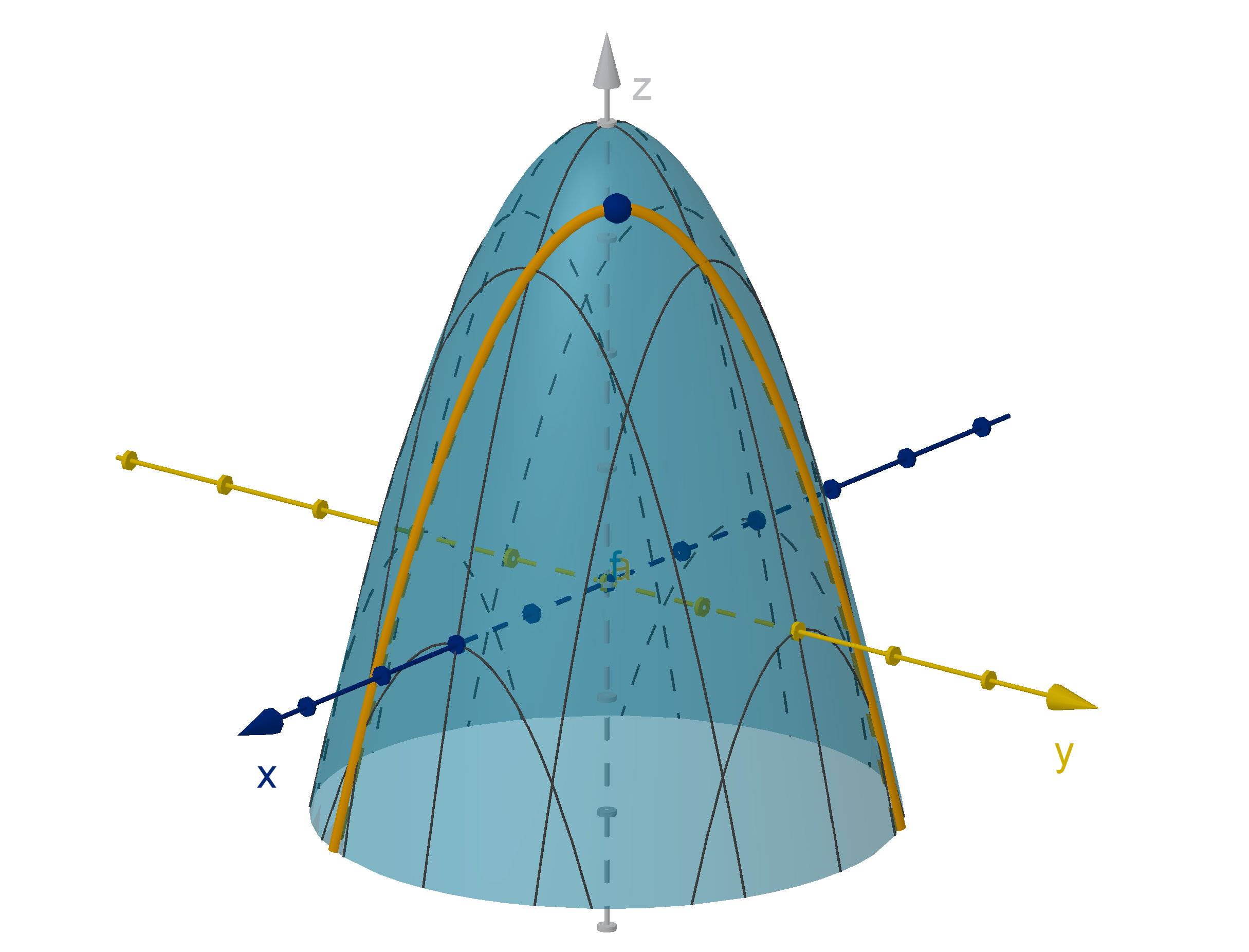
Figure: Maximizing f such that
x + y = 1
457
Question 5.7.2
How Do We Solve a Constrained Optimization?
The method of Lagrange Multipliers makes use of the following
theorem.
Theorem
Suppose an objective function f (x, y ) and a constraint function
g(x, y) are differentiable. The local extremes of f (x, y) given the
constraint g(x, y) = c occur where
∇f = λ∇g
for some number λ, or else where ∇g = 0. The number λ is called a
Lagrange Multiplier.
This theorem generalizes to functions of more variables.
458
Question 5.7.2
How Do We Solve a Constrained Optimization?
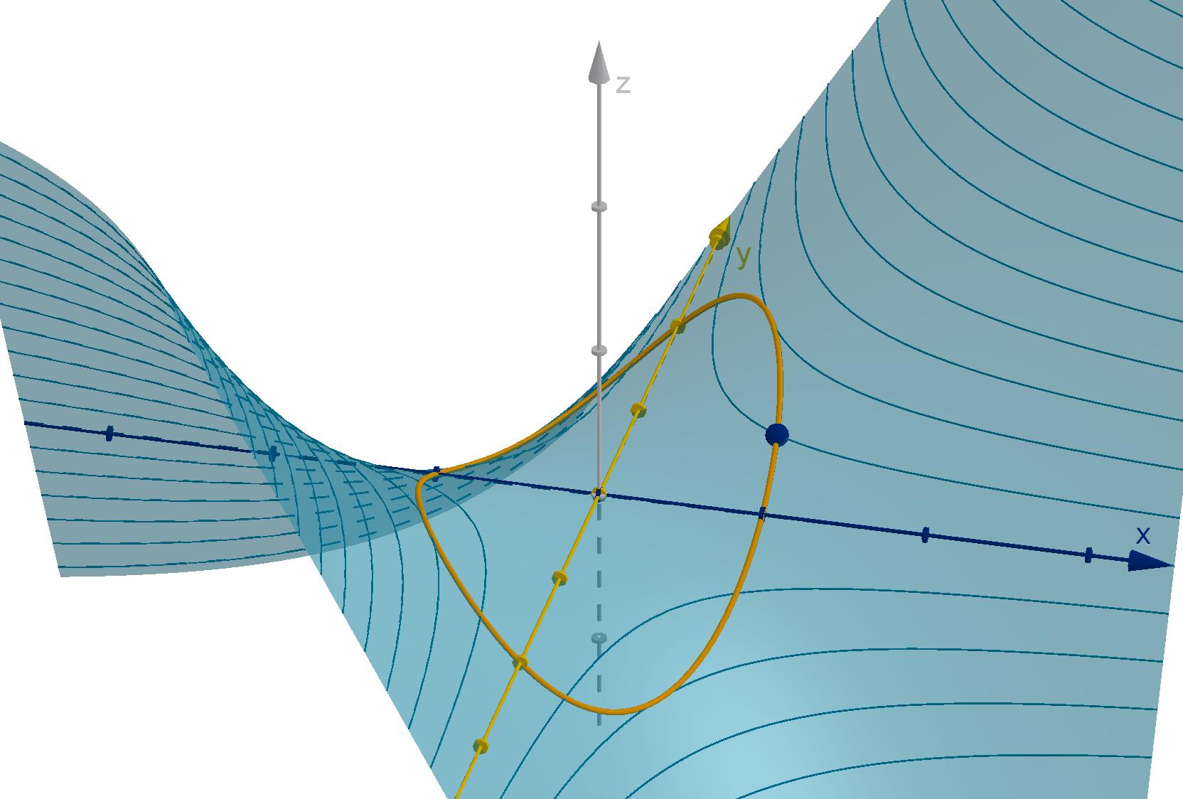
Figure: Where ∇f is not parallel to ∇g, we can travel along g(x, y ) = c and
increase the value of f . This is because D
u
f > 0 for some
u along the
constraint.
459
Example 5.7.3
The Maximum on a Curve
Find the point(s) on the ellipse 4x
2
+ y
2
= 4 on which the function
f (x, y) = xy is maximized.
460
Example 5.7.3
The Maximum on a Curve
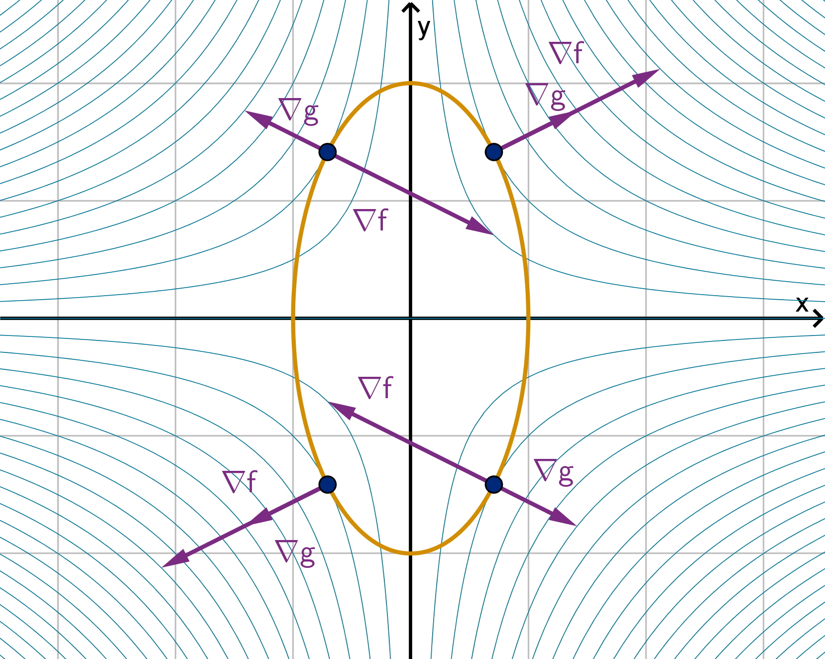
Figure: The four points that satisfy ∇f = λ∇g and g (x, y) = c.
Main Idea
The level set of a continuous (constraint) function is always closed. If it
is also bounded and the objective function is differentiable, then one of
the points produced by Lagrange multipliers will be the global maximum
and one will be the global minimum of the constrained optimization.
461
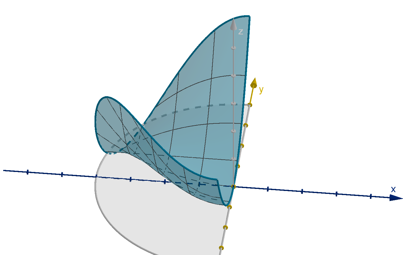
Example 5.7.4
The Maximum on a Surface
Find the maximum value of the function f (x, y , z) = x
4
y
4
z on the
sphere x
2
+ y
2
+ z
2
= 36.
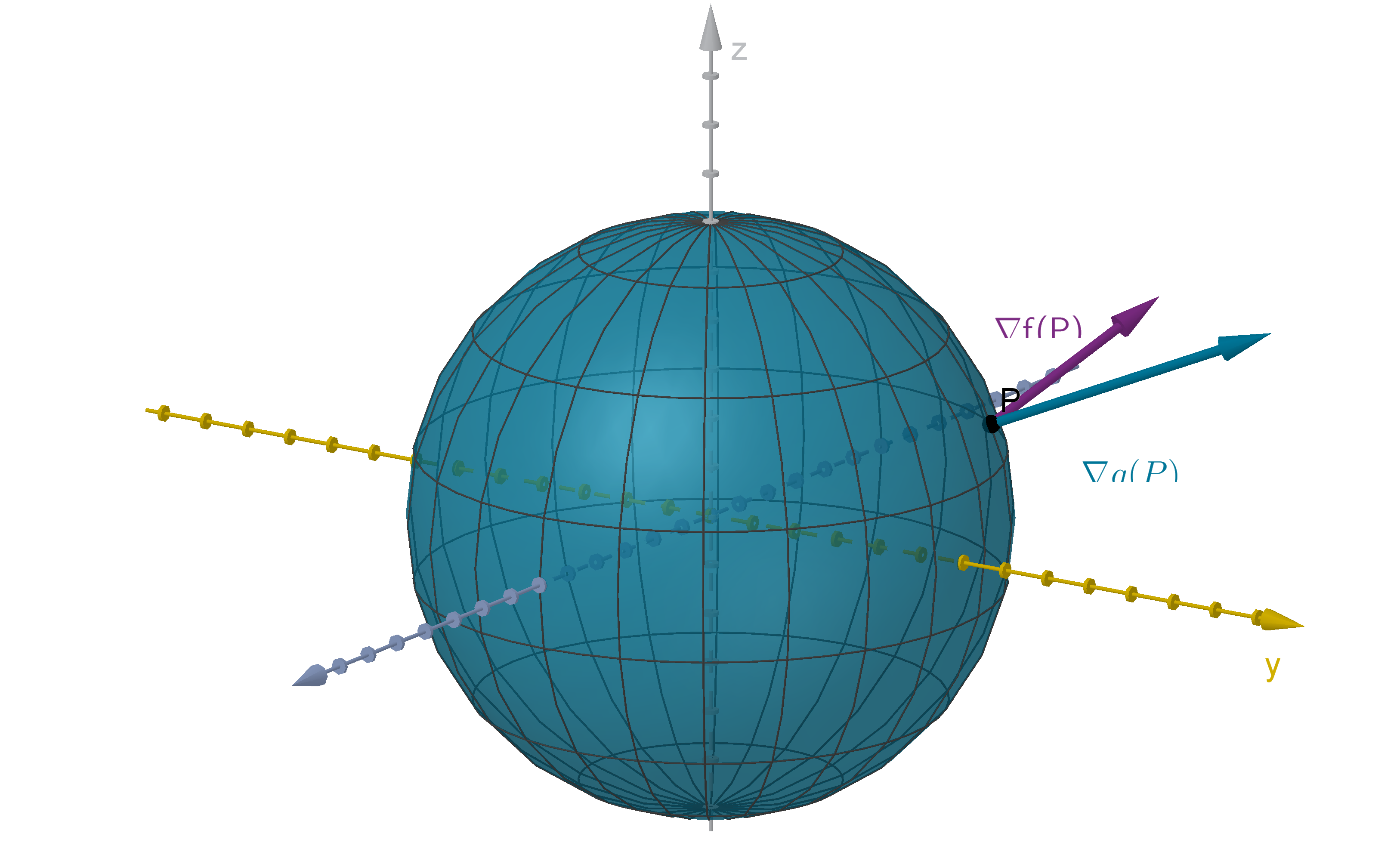
Figure: The gradient vector and level surface of a constraint function and the
gradient vector of the objective function
462
Synthesis 5.7.5
Using the Extreme Value Theorem and Lagrange Multipliers
How can Lagrange multipliers help us find the maximum of
f (x, y) = x
2
+ 2y
2
− x
2
y on the domain
D = {(x, y) : x
2
+ y
2
≤ 16, x ≤ 0}?
463
Synthesis 5.7.5
Using the Extreme Value Theorem and Lagrange Multipliers
Main Idea
To find the absolute minimum and maximum of a differentiable function
f (x, y) over a closed and bounded domain D:
1 Compute ∇f and find the critical points inside D.
2 Identify the boundary components. Find the critical points on each
using substitution or Lagrange multipliers.
3 Identify the endpoints (intersections) of the boundary components.
4 Evaluate f (x, y) at all of the above. The minimum is the lowest
number, the maximum is the highest.
464
Question 5.7.7
Can This Lagrange Apply to More Than One Constraint?
If we have two constraints in three-space, g (x, y, z) = c and
h(x, y, z) = d, then their intersection is generally a curve.
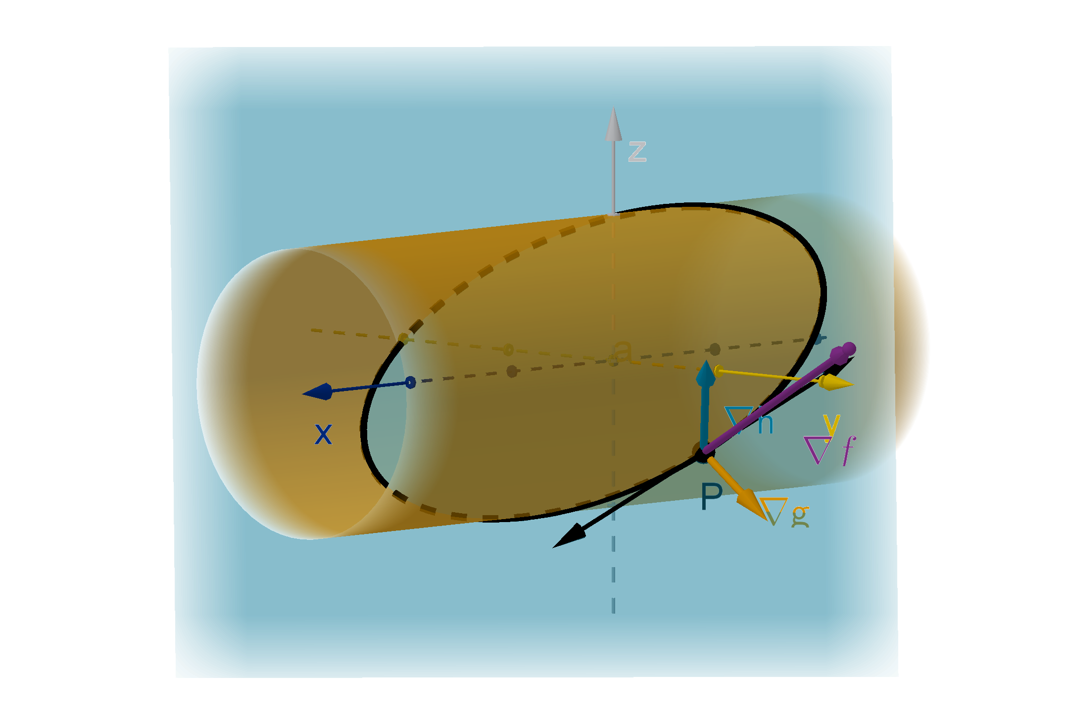
Figure: The intersection of the constraints g (x , y, z) = c and h(x, y, z) = d
465
Question 5.7.7
Can This Lagrange Apply to More Than One Constraint?
According to our earlier argument about directional derivatives, at a
maximum P on the constraint, ∇f (P) must be normal to the constraint.
There are more ways for this to happen with two constraint equations.
1 ∇f (P) could be parallel to ∇g (P).
2 ∇f (P) could be parallel to ∇h(P).
3 ∇f (P) could be the vector sum of a vector parallel to ∇g(P) and a
vector parallel to ∇h (P).
466
Question 5.7.7
Can This Lagrange Apply to More Than One Constraint?
Theorem
If f (x, y, z) is a differentiable function and g (x, y , z) = c and
h(x, y, z) = d are two constraints. If P is a maximum of f (x, y, z)
among the points that satisfy these constraints then either
∇f (P) = λ∇g (P) + µ∇h(P)
for some scalars λ and µ, or ∇g(P) and ∇h(P) are parallel.
This system of equations is usually difficult to solve by hand.
467
Question 5.7.7
Can This Lagrange Apply to More Than One Constraint?
Remark
You can check the reasonableness of this method by noting that it gives
us a system of 5 variables, x, y , z, λ, µ, and five equations:
f
x
(x, y , z) = λg
x
(x, y , z) + µh
x
(x, y , z) g(x, y, z) = c
f
y
(x, y , z) = λg
y
(x, y , z) + µh
y
(x, y , z) h(x, y, z) = d
f
z
(x, y , z) = λg
z
(x, y , z) + µh
z
(x, y , z)
We therefore generally expect this system to have a finite number of
solutions, though there are plenty of counterexamples to this expectation.
468
Section 5.7
Summary Questions
Q1 What is a constraint?
Q2 What equations do you write when you apply the method of
Lagrange multipliers?
Q3 Is the set of points that satisfies a constraint closed and bounded?
Explain.
Q4 How does a constraint arise when finding the maximum over a
closed and bounded domain?
469
Section 5.7
Q8
Suppose the curve below is the graph of g(x, y ) = k. Use methods from
calculus to find and mark the approximate location of the point that
maximizes the function f (x, y) = 3y − x subject to the constraint
g(x, y) = k. Justify your reasoning in a few sentences.
470
Section 5.7
Q10
Show that (3, 3) is not a local maximum of
f (x, y) = 2x
2
− 4xy + y
2
− 8x on the graph x
3
+ y
3
= 6xy.
471
Section 5.7
Q18
Consider the following two questions:
Find the maximum value of f (x, y) that satisfies x
2
+ y
2
≤ 9.
Find the maximum value of f (x, y) that satisfies x
2
+ y
2
= 9.
a How are the questions different?
b Which question takes less work to solve? Explain how you know.
c Do solutions exist to both questions? What additional information
would guarantee that they do?
472
Section 5.7
Q20
Consider the function f (x, y) = x
2
+ 6xy + 9y
2
+ 5. Find the maximum
and minimum values of f on the domain
D = {(x, y) : y ≥ x, x ≥ 0, x
2
+ y
2
≤ 10}
473