Section 4.1
Three-Dimensional Coordinate Systems
Goals:
1 Plot points in a three-dimensional coordinate system.
2 Use the distance formula.
3 Recognize the equation of a sphere and find its radius and center.
4 Graph an implicit function with a free variable.
Question 4.1.1
How Do Cartesian Coordinates Extend to Higher Dimensions?
Recall how we constructed the Cartesian plane.
x
y
y
−4
−4
−3
−3
−2
−2
−1
−1
1
1
2
2
3
3
4
4
(2, 0)
(2, 3)
1 Assign origin and two directions (x, y).
2 y is 90 degrees anticlockwise from x.
3 Axes consist of the points displaced in
only one direction.
4 Coordinates refer to displacement from
the origin in each direction.
5 Either displacement can happen first.
6 Each point has exactly one ordered
pair that refers to it.
251
Question 4.1.1
How Do Cartesian Coordinates Extend to Higher Dimensions?
In a three-dimensional Cartesian coordinate system. We can extrapolate
from two dimensions.
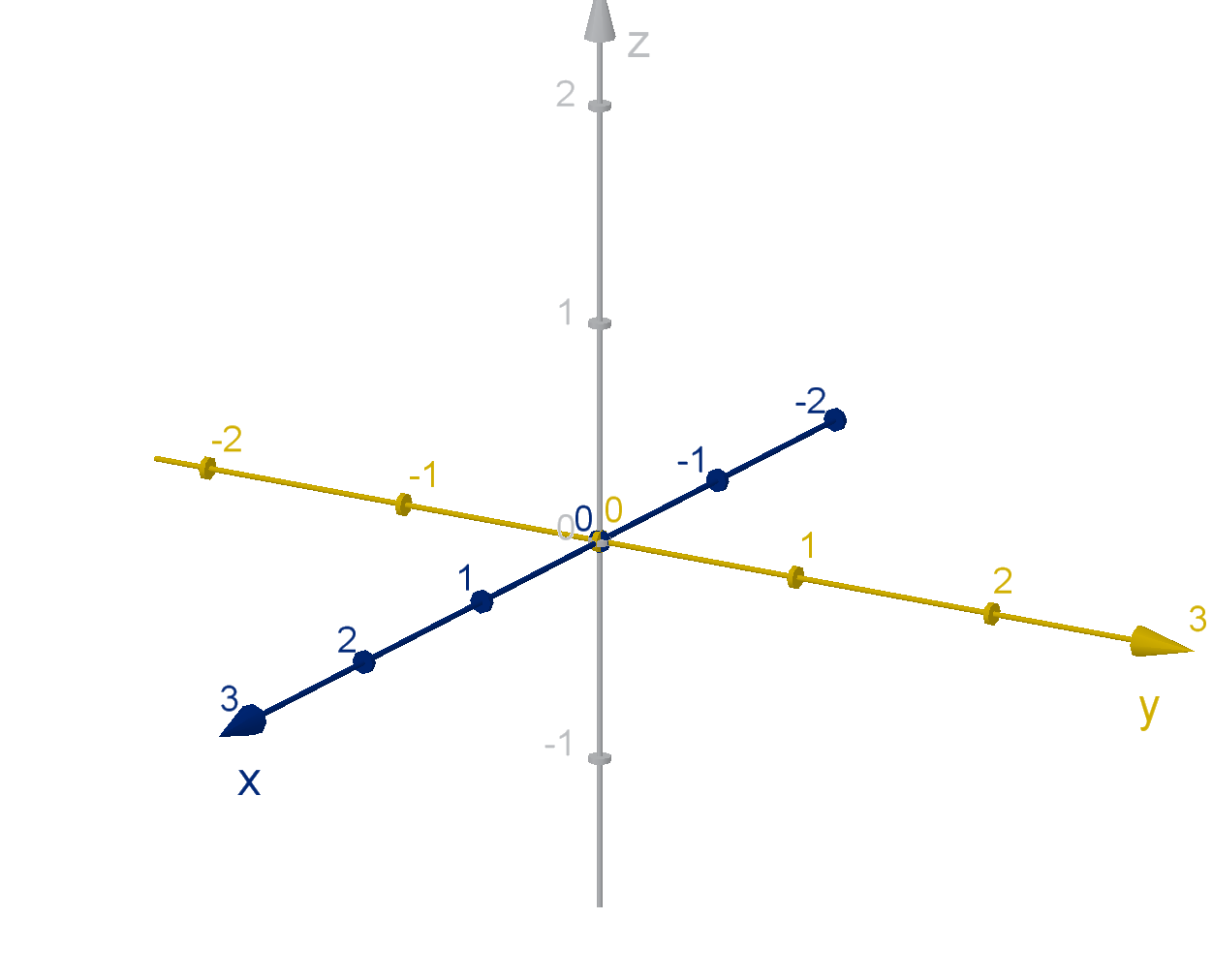
1 Assign origin and three
directions (x, y, z).
2 Each axis makes a 90 degree
angle with the other two.
3 The z direction is determined
by the right-hand rule.
252
Question 4.1.2
How Do We Establish Which Direction Is Positive in Each Axis?
The right hand rule says that if you make the fingers of your right hand
follow the (counterclockwise) unit circle in the xy-plane, then your
thumb indicates the direction of the positive z-axis.
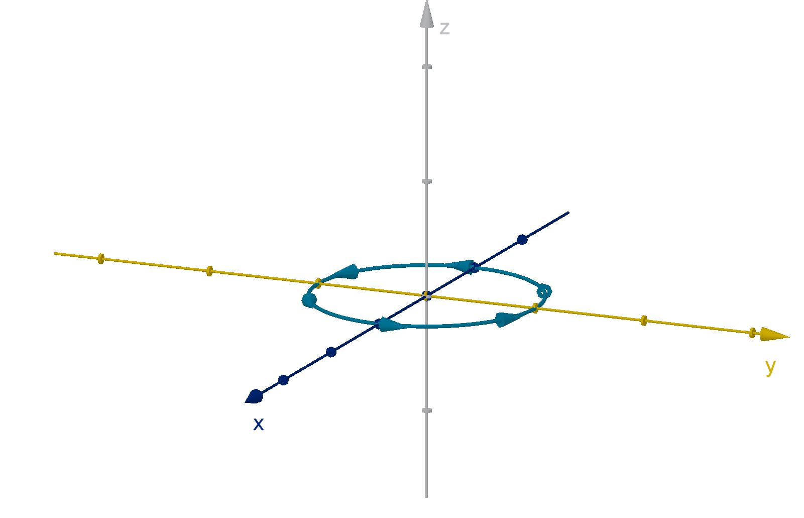
Figure: The counterclockwise unit circle in the xy-plane
253
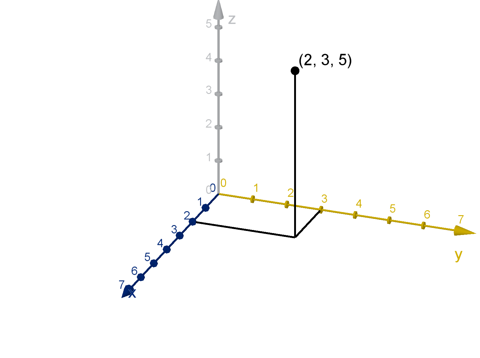
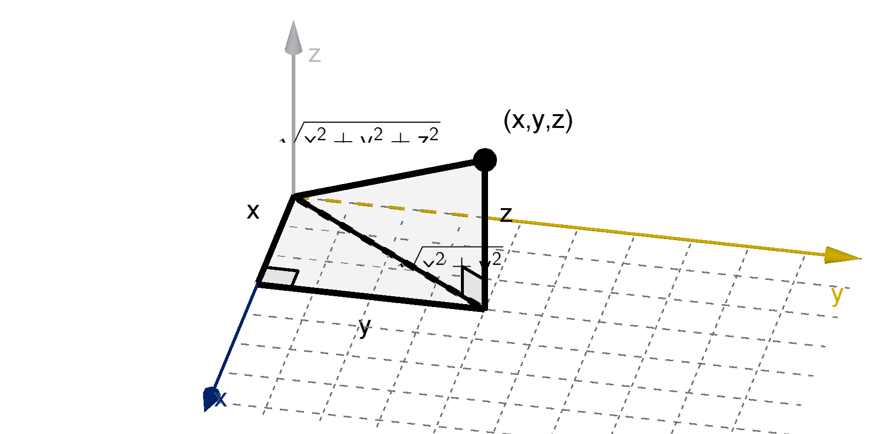
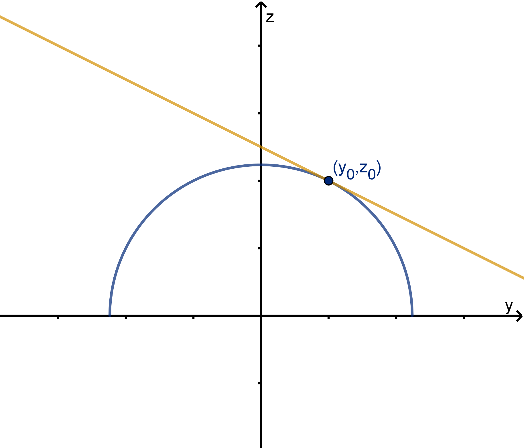
Example 4.1.3
Drawing a Location in Three-Dimensional Coordinates
The point (2, 3, 5) is the point displaced from the origin by
2 in the x direction
3 in the y direction
5 in the z direction.
How do we draw a reasonable diagram of where this point lies?
254
Example 4.1.3
Drawing a Location in Three-Dimensional Coordinates
The point (2, 3, 5) is the point displaced from the origin by
2 in the x direction
3 in the y direction
5 in the z direction.
How do we draw a reasonable diagram of where this point lies?
254
Example 4.1.3
Drawing a Location in Three-Dimensional Coordinates
How can we draw a reasonable diagram of (−5, 1, −4)?
255
Example 4.1.3
Drawing a Location in Three-Dimensional Coordinates
How can we draw a reasonable diagram of (−5, 1, −4)?
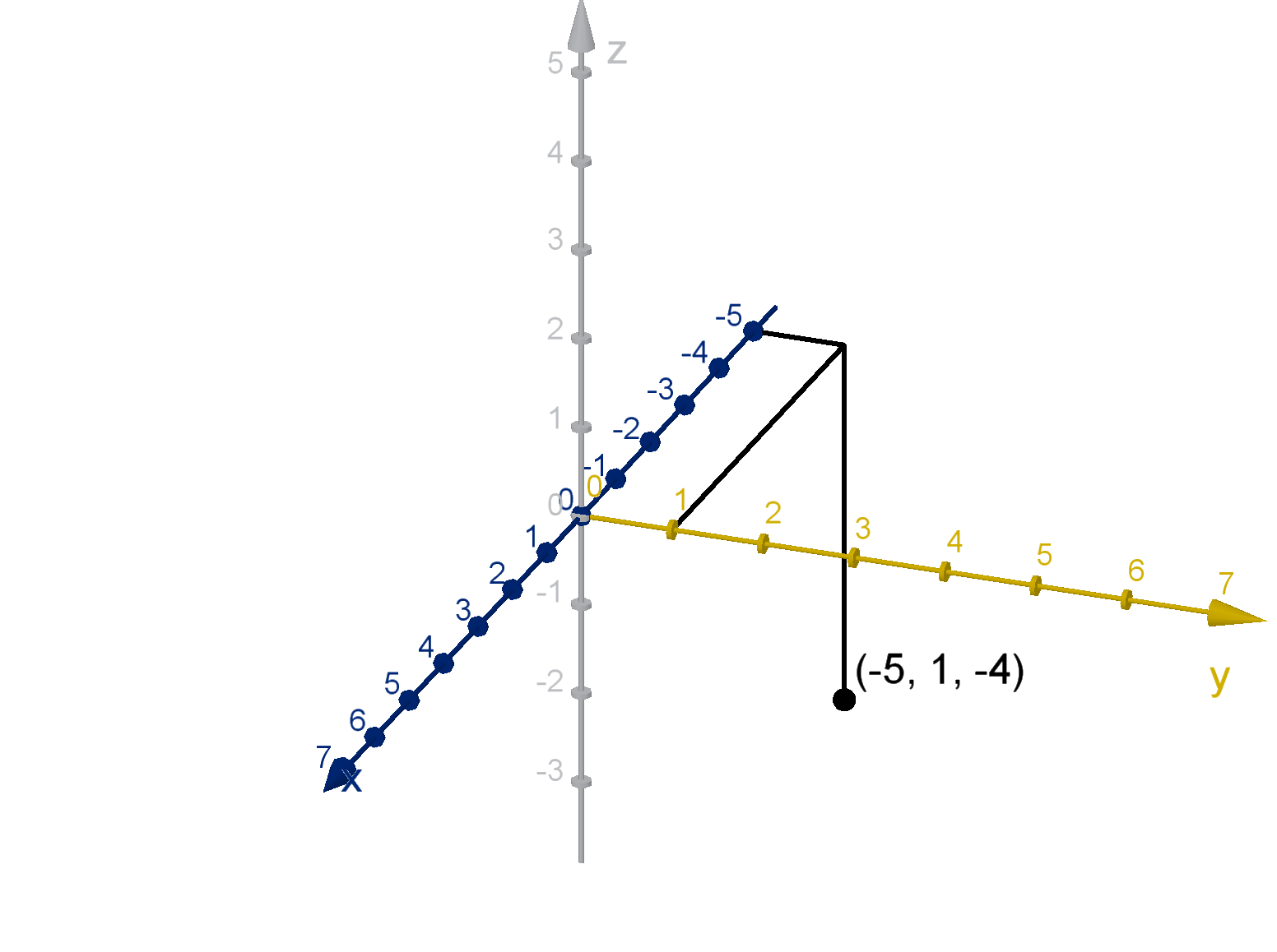
255
Question 4.1.4
How Do We Measure Distance in Three-Space?
Theorem
The distance from the origin to the point (x, y , z) is given by the
Pythagorean Theorem
D =
p
x
2
+ y
2
+ z
2
256
Question 4.1.4
How Do We Measure Distance in Three-Space?
Theorem
The distance from the point (x
1
, y
1
, z
1
) to the point (x
2
, y
2
, z
2
) is given
by
D =
q
(x
1
− x
2
)
2
+ (y
1
− y
2
)
2
+ (z
1
− z
2
)
2
257
Question 4.1.5
What Is a Graph?
Definition
The graph of an implicit equation is the set of points whose coordinates
satisfy that equation. In other words, the two sides are equal when we
plug the coordinates in for x, y and z.
Example
The graph of
x
2
+ (y − 4)
2
+ (z + 1)
2
= 9
is the set of points that are distance 3
from the point (0, 4, −1)
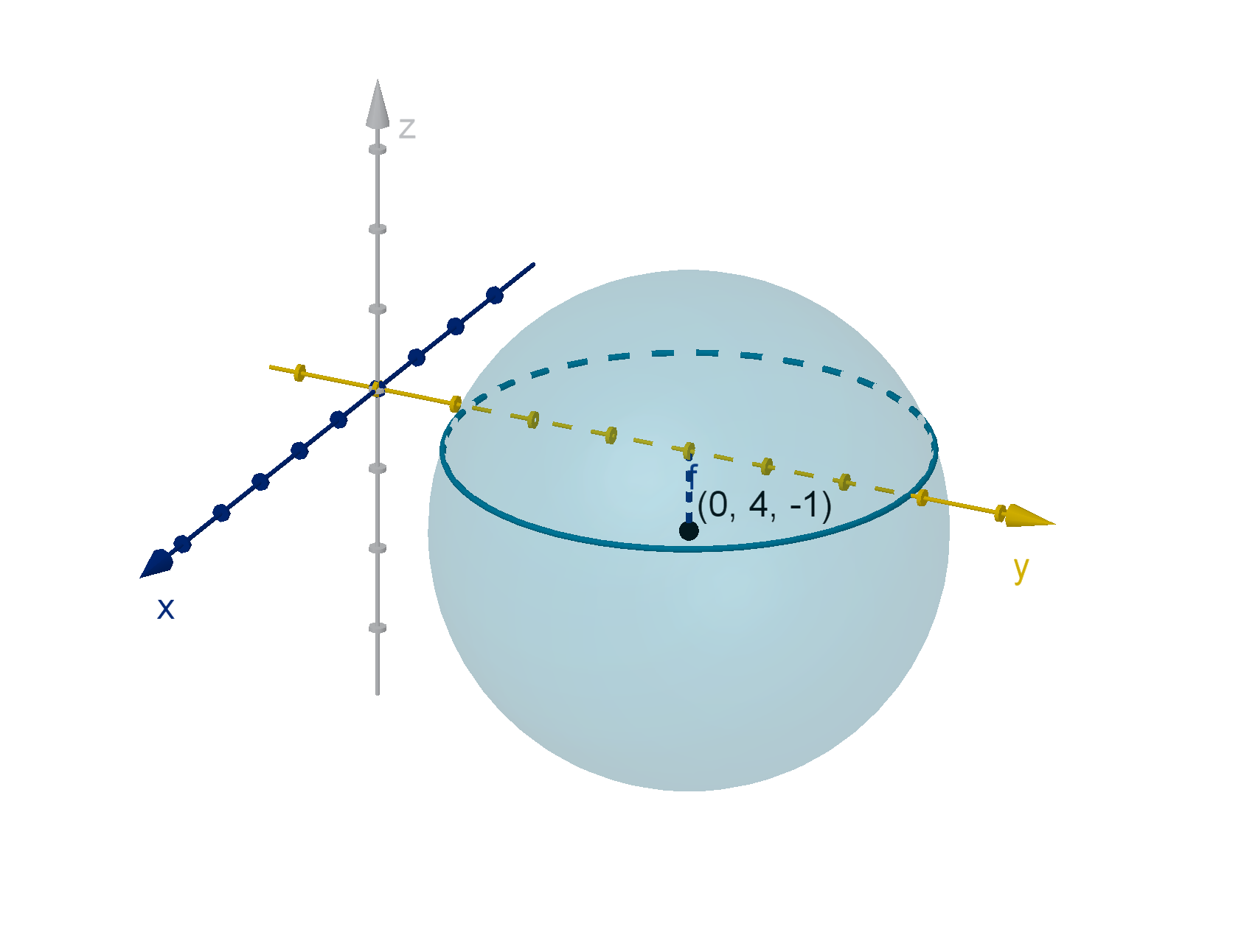
258
Example 4.1.6
Graphing an Equation with Two Free Variables
Sketch the graph of the equation y = 3.
259
Example 4.1.6
Graphing an Equation with Two Free Variables
In addition to coordinate axes, 3-dimensional space has 3 coordinate
planes.
1 The graph of z = 0 is the xy -plane.
2 The graph of x = 0 is the yz-plane.
3 The graph of y = 0 is the xz-plane.
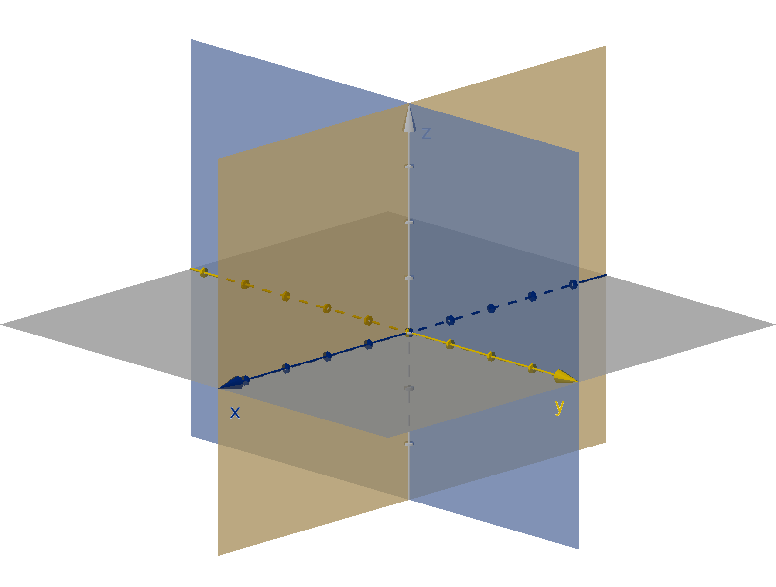
Figure: The coordinate planes in 3-dimensional space.
260
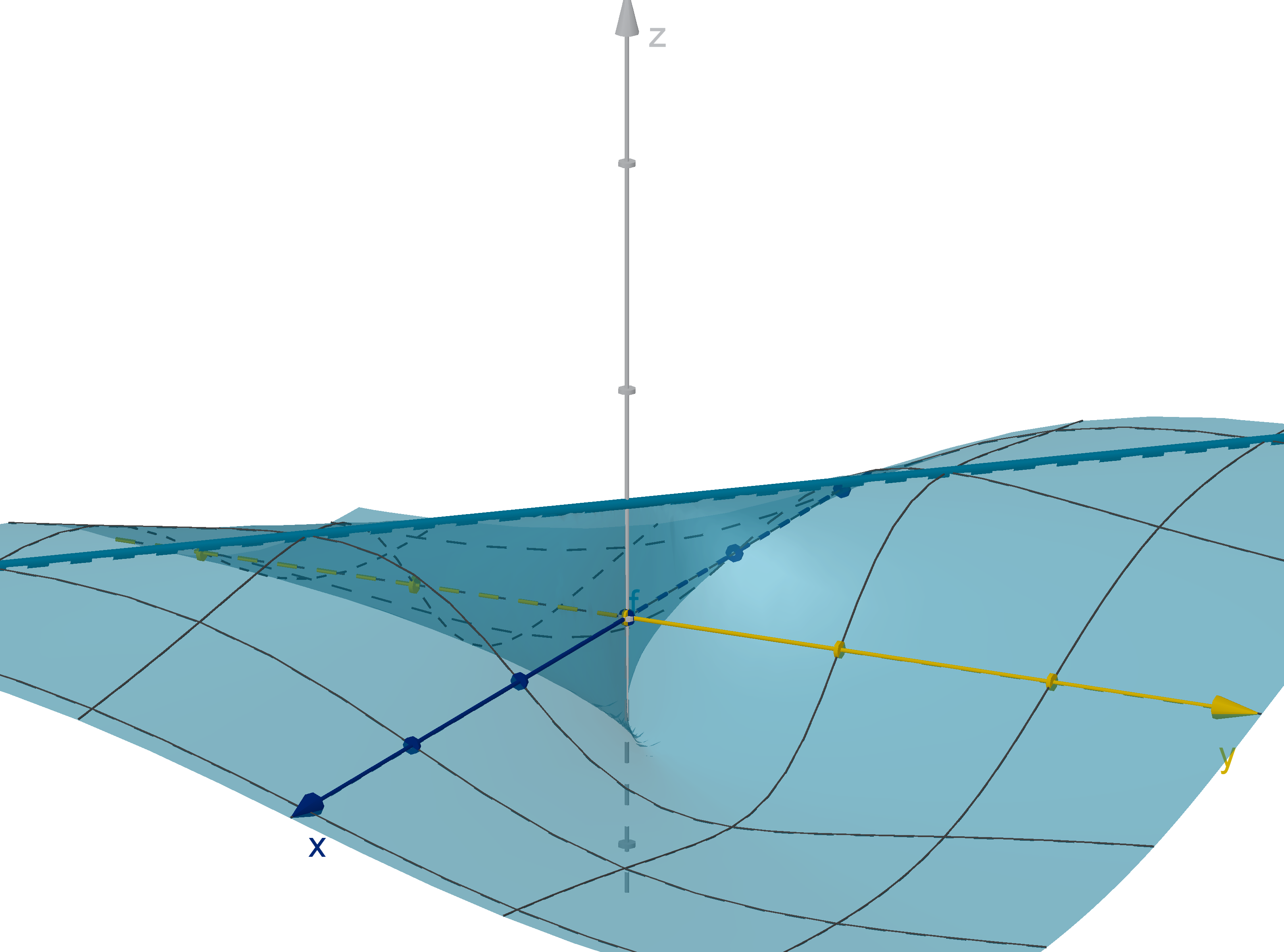
Example 4.1.7
Graphing an Equation with One Free Variable
Sketch the graph of the equation z = x
2
− 3.
261
Question 4.1.8
What Do the Graphs of Implicit Equations Look Like Generally?
Notice that the graph of an implicit equation in the plane is generally
one-dimensional (a curve), whereas the graph of an implicit equation in
three-space is generally two-dimensional (a surface).
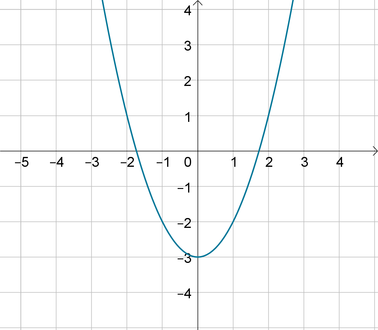
Figure: The curve y = x
2
− 3
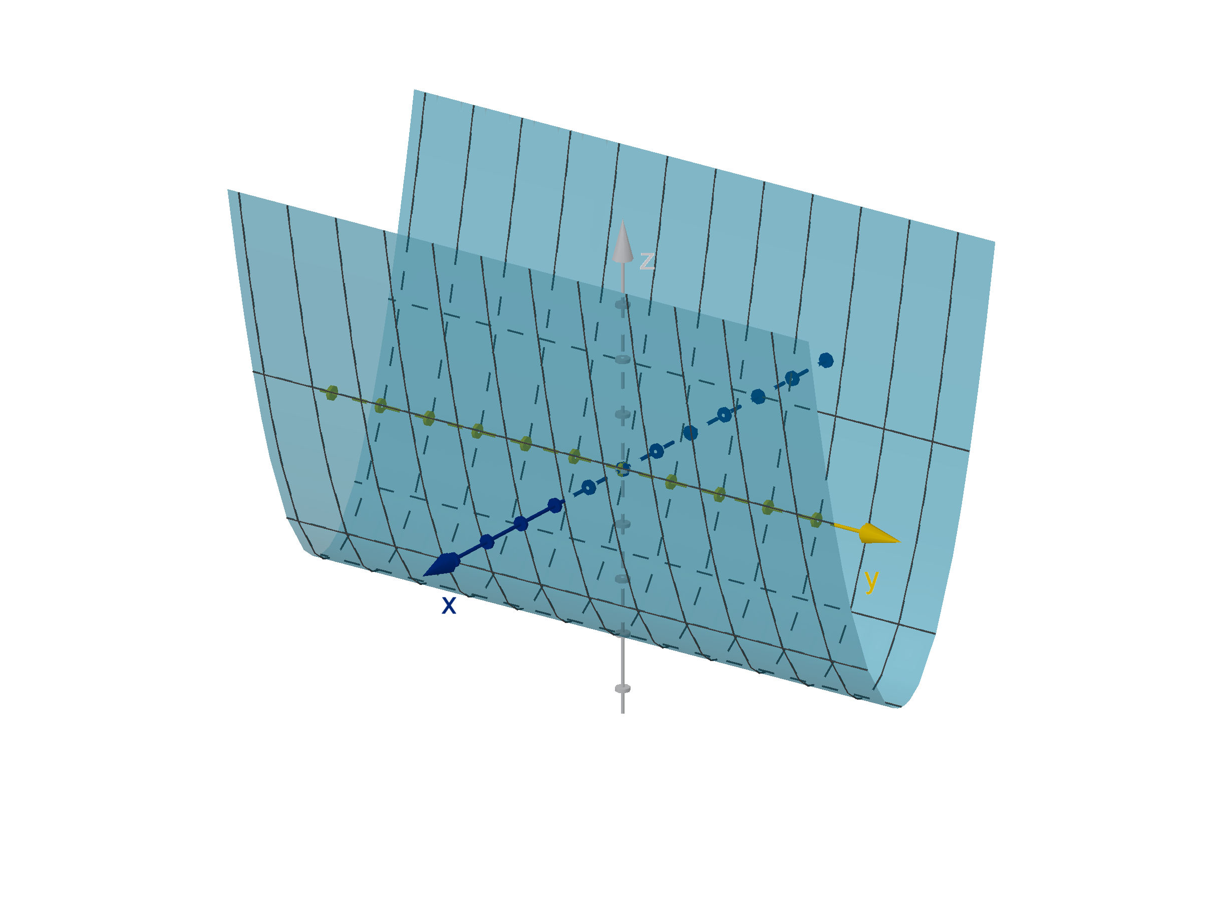
Figure: The surface z = x
2
− 3
262
Question 4.1.9
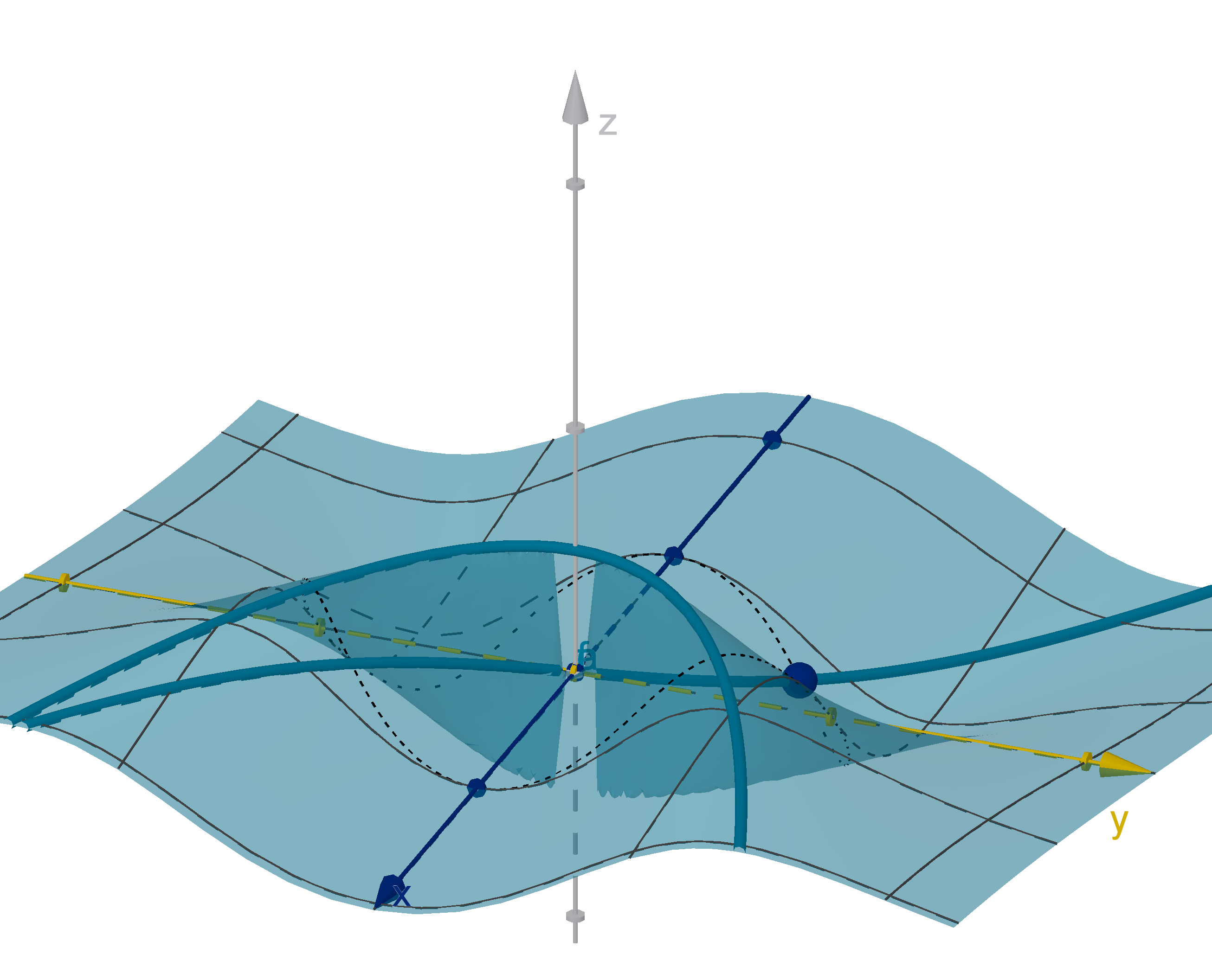
What Is the Slope-Intercept Equation of a Plane?
Unlike a line, a non-vertical plane has two slopes. One measures rise over
run in the x-direction, the other in the y -direction.
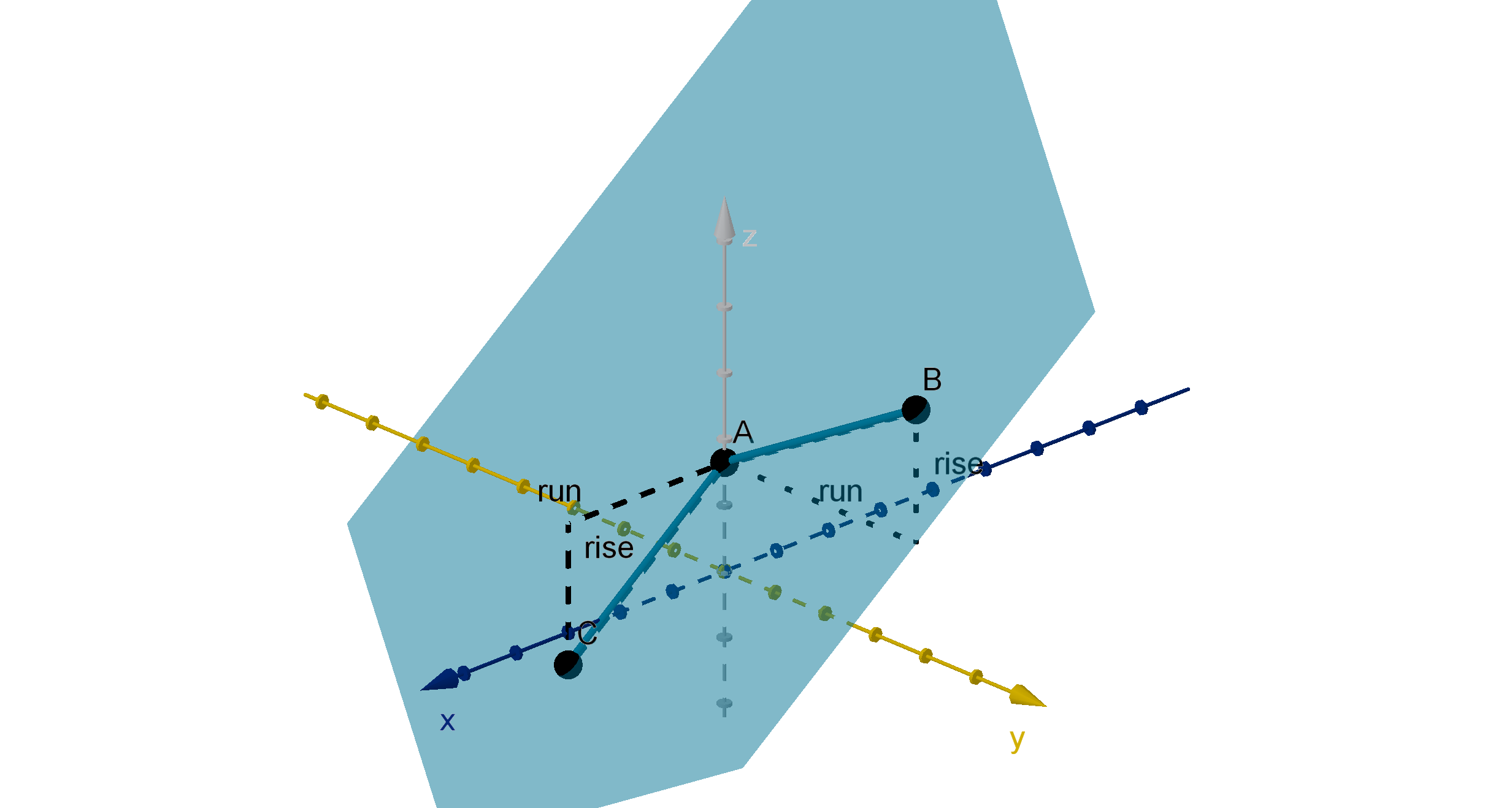
Figure: A plane with slopes in the x and y directions.
263
Question 4.1.9
What Is the Slope-Intercept Equation of a Plane?
Equation
A plane with z intercept (0, 0, b) and slopes m
x
and m
y
in the x and y
directions has equation
z = m
x
x + m
y
y + b.
264
Example 4.1.10
Writing the Equation of a Plane
Write the equation of a plane with intercepts (4, 0, 0), (0, 6, 0) and
(0, 0, 8).
265
Example 4.1.10
Writing the Equation of a Plane
Main Idea
Given three points in a plane A = (x
1
, y
1
, z
1
), B = (x
2
, y
2
, z
2
) and
C = (x
3
, y
3
, z
3
)
1 If two points share an x-coordinate, we can directly compute m
y
and vice versa.
2 Failing that, we can set up a system of equations and solve for m
x
,
m
y
and b.
266
Question 4.1.11
How Do We Extrapolate to Even Higher Dimensions?
We can use a coordinate system to describe a space with more than 3
dimensions. k-dimensional space can be defined as the set of points of
the form
P = (x
1
, x
2
, . . . , x
k
).
Theorem
The distance from the origin to P = (x
1
, x
2
, . . . , x
k
) in k-space is
q
x
2
1
+ x
2
2
+ ··· + x
2
k
There is no right hand rule for higher dimensions, because we can’t draw
these spaces anyway.
267
Section 4.1
Summary Questions
Q1 What displacements are represented by the notation (a, b, c)?
Q2 What is the right hand rule and what does it tell you about a
three-dimensional coordinate system?
Q3 In three-space, what is the y-axis? What are the coordinates of a
general point on it?
Q4 In three space, what is the xz-plane? What are the coordinates of a
general point on it? What is its equation?
Q5 How do we use a free variable to sketch a graph?
Q6 How do we recognize the equation of a sphere?
268
Section 4.1
Q11
Draw diagrams of points with the following coordinates.
a (6, 1, 2)
b (−3, 0, 0)
c (2, −1, 4)
d (0, 3, 5)
269
Section 4.1
Q11
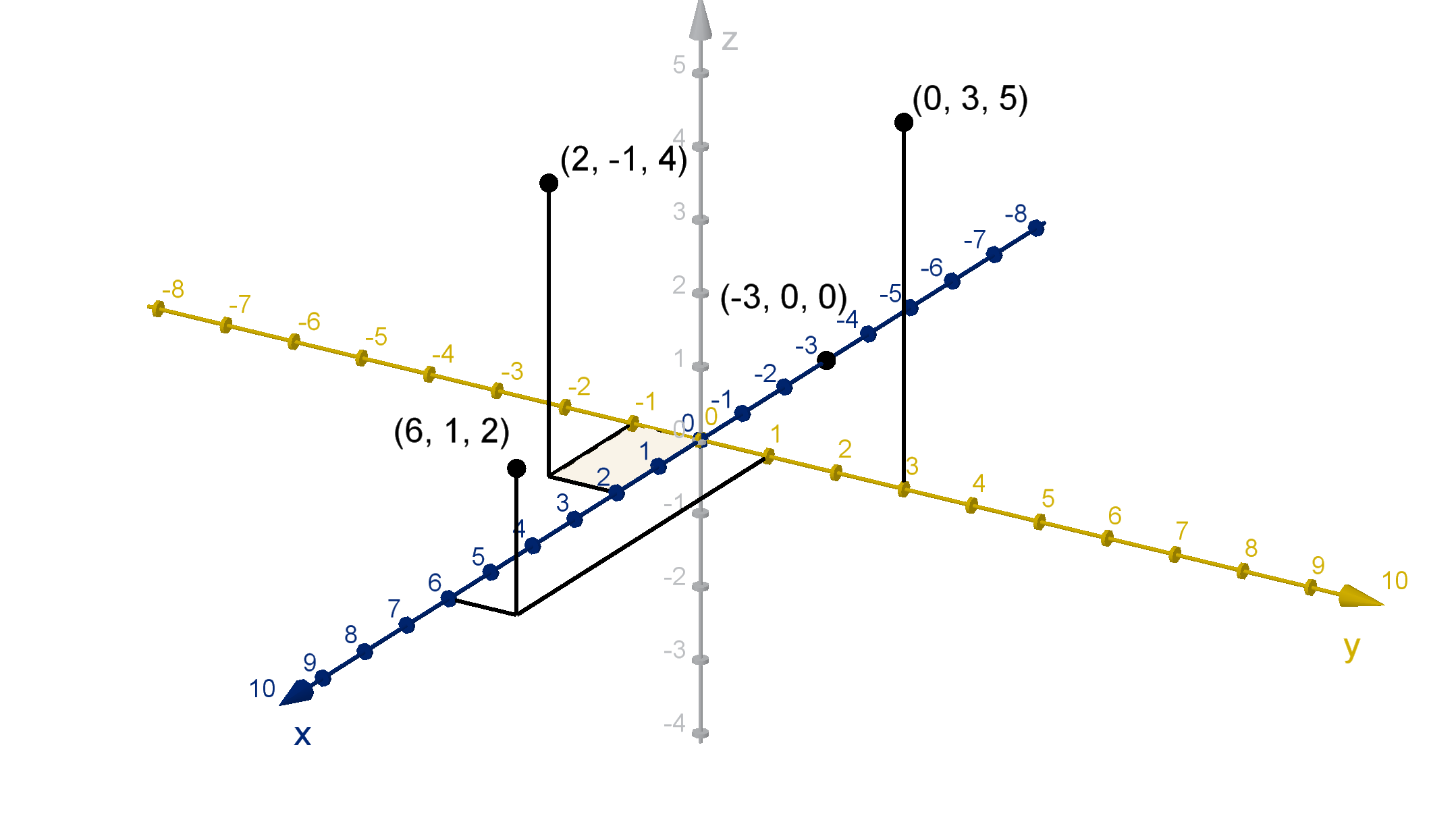
269
Section 4.1
Q50
The graph of x
2
+ y
2
= 0 in R
2
is a point, not a curve. Use this idea to
write an equation for the intersection of the graphs f (x, y, z) = c and
g(x, y, z) = d . What do you expect the dimension of this intersection to
be?
270
Section 4.1
Q34
Gabby is trying to find the equation of a plane P, but she doesn’t know
any points on the xz-plane or yz-plane. Instead she knows that P
contains the points:
A = (1, 3, 6) B = (5, 3, 4) C = (7, 5, 10)
Using points A and B, she decides that m
x
=
4−6
5−1
= −
1
2
. Using points A
and C , she decides that m
y
=
10−6
5−3
= 2.
a Which of Gabby’s conclusions do you agree with and which do you
disagree with? Why?
b How could you fix the one that is wrong?
271
Section 4.1
Q36
Recall that we can write the equation of a line in R
2
in point-slope form:
y − y
0
= m(x − x
0
)
where m is the slope and (x
0
, y
0
) is a known point. This was especially
useful in single-variable calculus for writing equations of tangent lines.
a How would you expect to write the equation of the plane P through
(2, 4, −6) with slopes m
x
=
1
2
and m
y
= −3?
b Does your answer to a actually pass through (2, 4, −6)? How do
you know?
c Is your answer to a actually the equation of a plane? How do you
know? Does it have the correct slopes?
d Write a general expression for point-slope form for a plane.
272
Section 4.1
Q36
a How would you expect to write the equation of the plane P through
(2, 4, −6) with slopes m
x
=
1
2
and m
y
= −3?
272
Section 4.1
Q36
b Does your answer to a actually pass through (2, 4, −6)? How do
you know?
272
Section 4.1
Q36
c Is your answer to a actually the equation of a plane? How do you
know? Does it have the correct slopes?
272
Section 4.1
Q36
d Write a general expression for point-slope form for a plane.
272
Section 4.2
Functions of Several Variables
Goals:
1 Convert an implicit function to an explicit function.
2 Calculate the domain of a multivariable function.
3 Calculate level curves and cross sections.
Question 4.2.1
What Is a Function of More than One Variable?
Definition
A function of two variables is a rule that assigns a number (the output)
to each ordered pair of real numbers (x, y ) in its domain. The output is
denoted f (x, y).
Some functions can be defined algebraically. If
f (x, y) =
p
36 −4x
2
− y
2
then
f (1, 4) =
p
36 −4 · 1
2
− 4
2
= 4.
274
Example 4.2.2
The Domain of a Function
Identify the domain of f (x, y) =
p
36 −4x
2
− y
2
.
Figure: The domain of a function
275
Example 4.2.2
The Domain of a Function
Identify the domain of f (x, y) =
p
36 −4x
2
− y
2
.
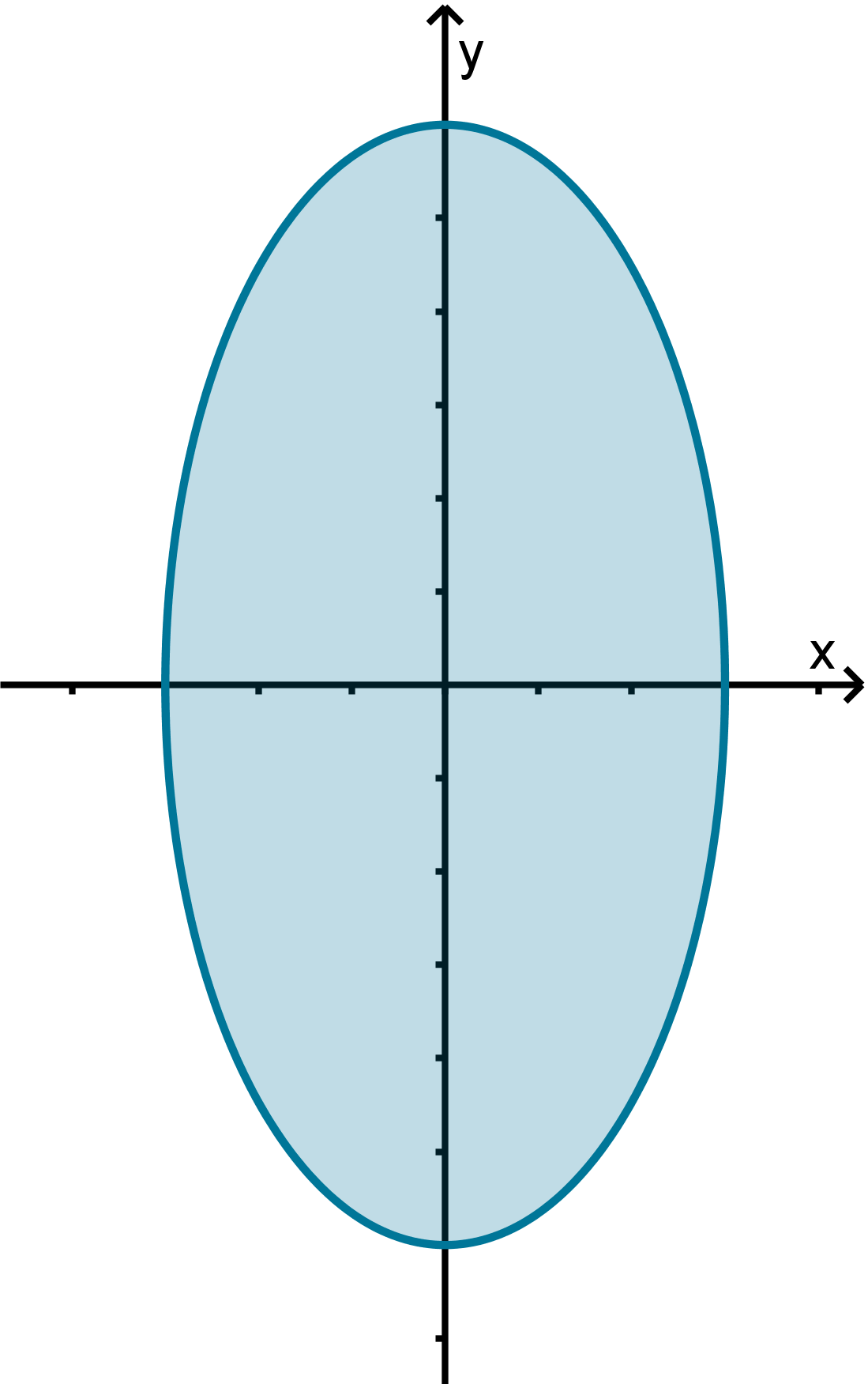
Figure: The domain of a function
275
Application 4.2.3
Temperature Maps
Many useful functions cannot be defined algebraically. There is a
function T (x, y) which gives the temperature at each latitude and
longitude (x, y) on earth.
T (−71.06, 42.36) = 50
T (−84.38, 33.75) = 59
T (−83.74, 42.28) = 41
Figure: A temperature map
276
Application 4.2.4
Digital Images
A digital image can be defined by a brightness function B(x, y).
y
x
687
1024
B(339, 773) = 158 B(340, 773) = 127
Figure: An image represented as a brightness function B on each pixel
277
Question 4.2.5
What Is the Graph of a Two-Variable Function?
Definition
The graph of a function f (x, y) is the set of all points (x, y , z) that
satisfy
z = f (x, y ).
The height z above a point (x, y ) represents the value of the function at
(x, y).
278
Question 4.2.5
What Is the Graph of a Two-Variable Function?
In this figure, f (1, 4) is equal to the height of the graph above (1, 4, 0).
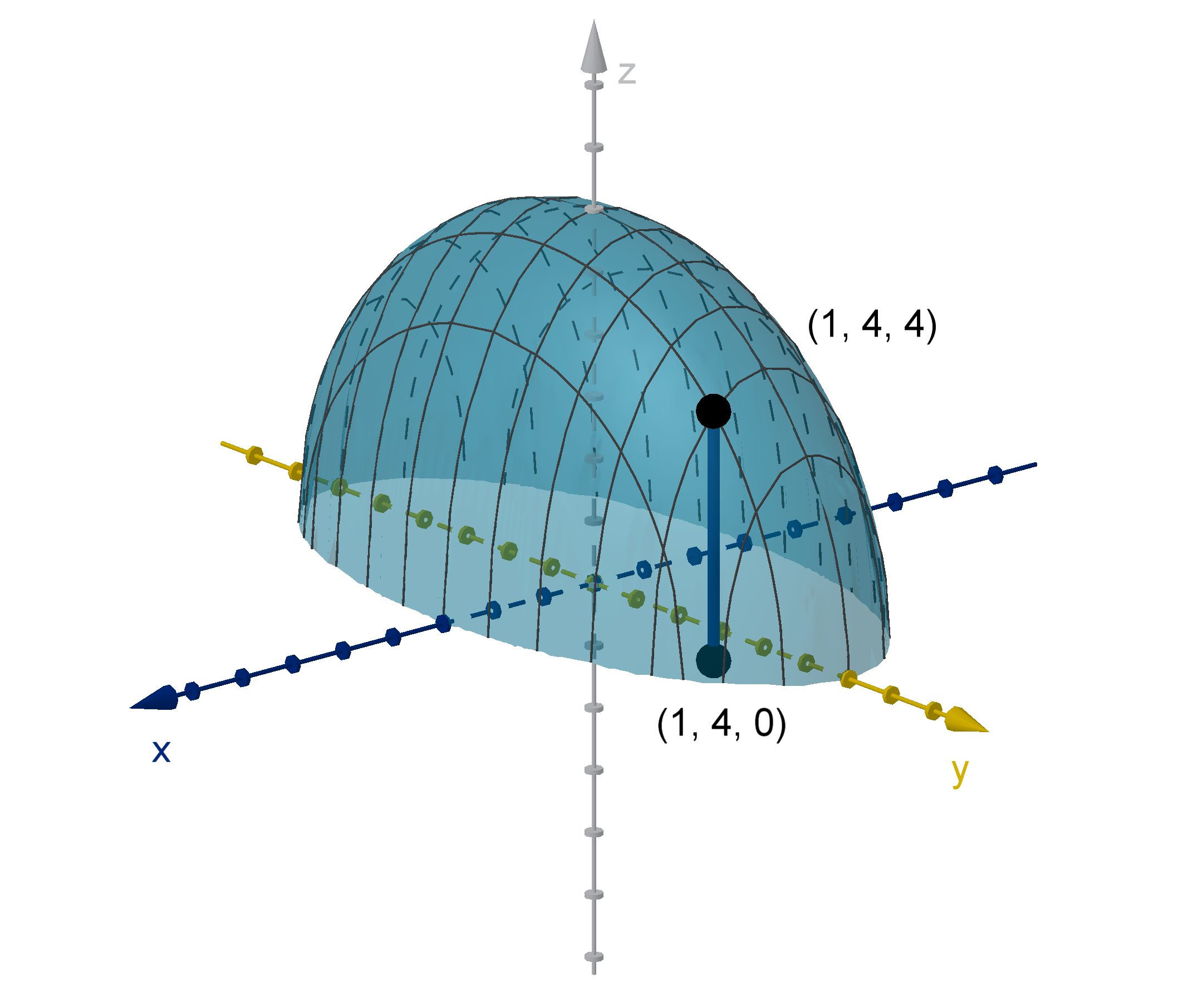
Figure: The graph z =
p
36 −4x
2
− y
2
279
Question 4.2.6
How Do We Visualize a Graph in Three-Space?
Definition
A level set of a function f (x, y) is the graph of the equation f (x, y ) = c
for some constant c. For a function of two variables this graph lies in the
xy-plane and is called a level curve.
Example
Consider the function
f (x, y) =
p
36 −4x
2
− y
2
.
The level curve
p
36 −4x
2
− y
2
= 4 simplifies
to 4x
2
+ y
2
= 20. This is an ellipse.
Other level curves have the form
p
36 −4x
2
− y
2
= c or 4x
2
+ y
2
= 36 −c
2
.
These are larger or smaller ellipses.

280
Question 4.2.6
How Do We Visualize a Graph in Three-Space?
Level curves take their shape from the intersection of z = f (x, y ) and
z = c. Seeing many level curves at once can help us visualize the shape
of the graph.
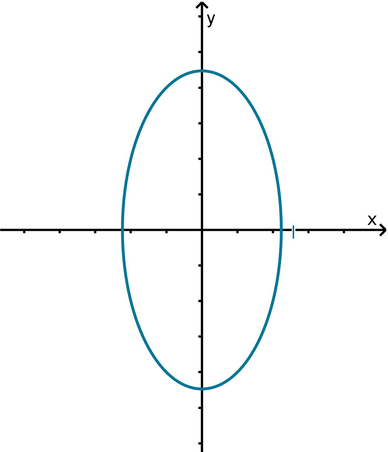
Figure: The graph z = f (x, y ), the planes z = c, and the level curves
281
Example 4.2.7
Drawing Level Curves
Where are the level curves on this temperature map?
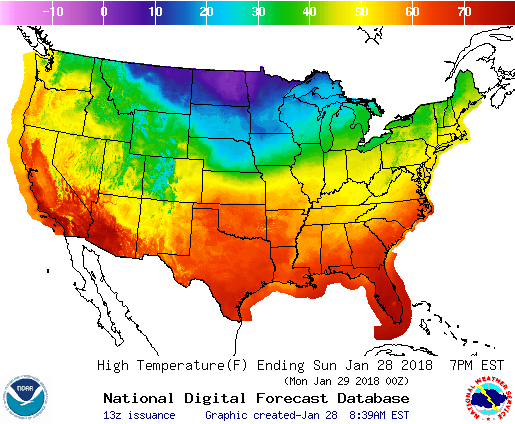
Figure: A temperature map
282
Example 4.2.8
Using Level Curves to Describe a Graph
What features can we discern from the level curves of this topographical
map?
Figure: A topographical map
283
Example 4.2.9
A Cross Section
Definition
The intersection of a plane with a graph is a cross section. A level curve
is a type of cross section, but not all cross sections are level curves.
Find the cross section of z =
p
36 −4x
2
− y
2
at the plane y = 1.
284
Example 4.2.9
A Cross Section
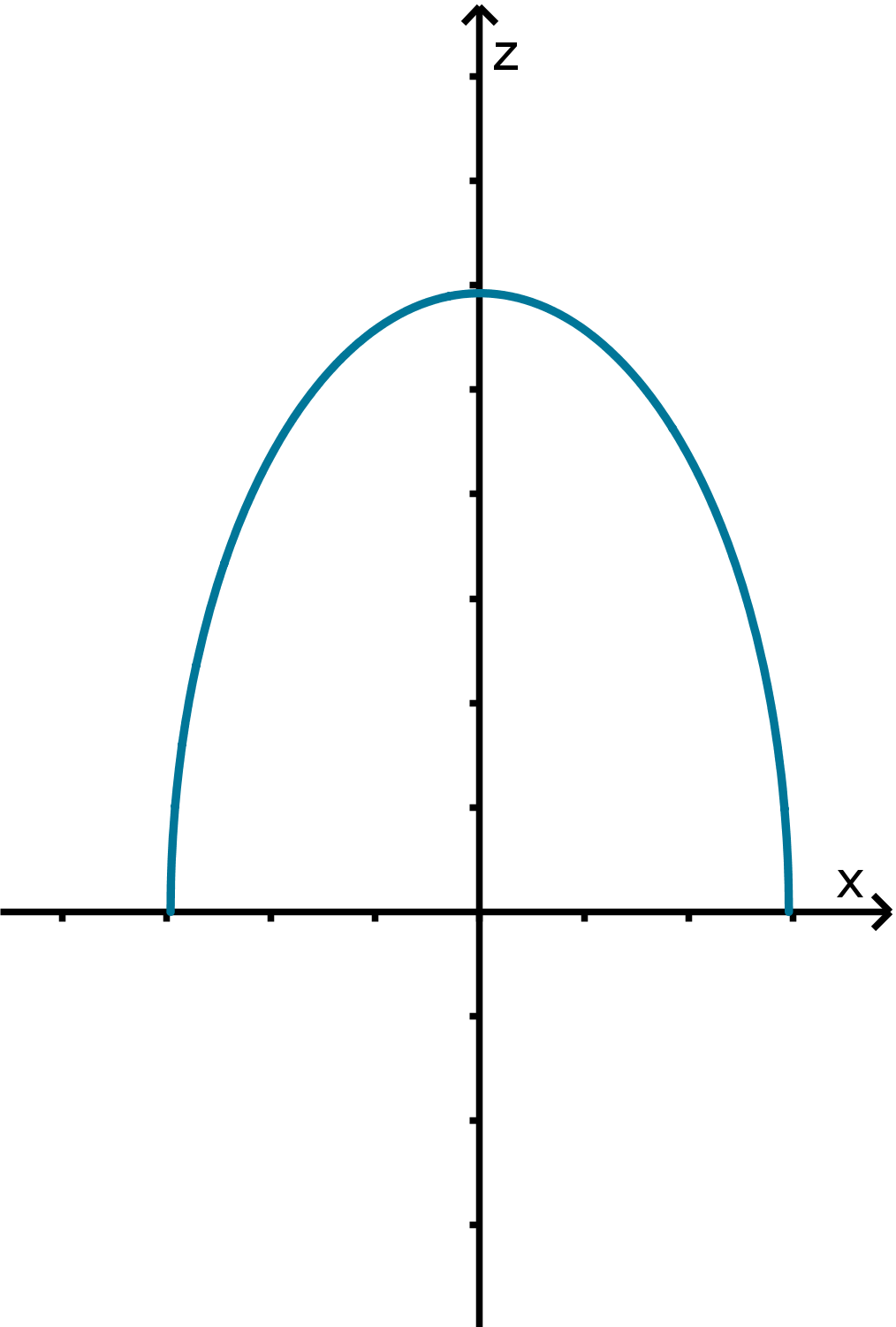
Figure: The y = 1 cross section of z =
p
36 −4x
2
− y
2
285
Example 4.2.10
Converting an Implicit Equation to a Function
Definition
We sometimes call an equation in x, y and z an implicit equation.
Often in order to graph these, we convert them to explicit functions of
the form z = f (x, y)
Write the equation of a paraboloid x
2
− y + z
2
= 0 as one or more
explicit functions so it can be graphed. Then find the level curves.
286
Example 4.2.10
Converting an Implicit Equation to a Function
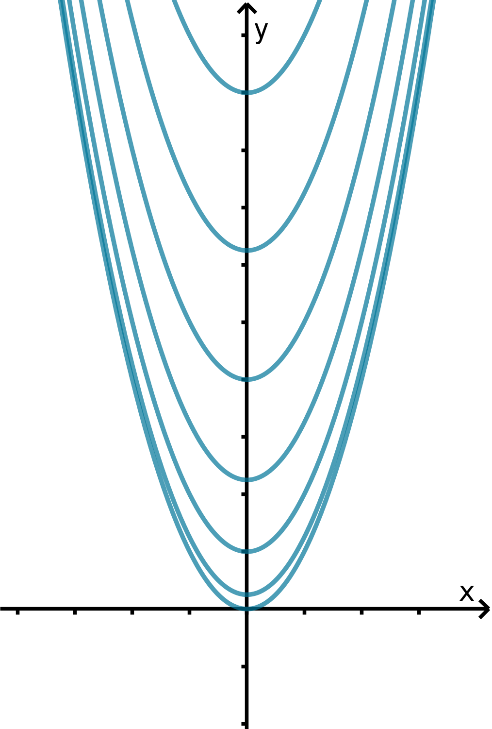
Figure: Level curves of x
2
− y + z
2
= 0
287
Question 4.2.11
How Does this Apply to Functions of More Variables?
We can define functions of three variables as well. Denoting them
f (x, y, z). For even more variables, we use x
1
through x
n
. The definitions
of this section can be extrapolated as follows.
Variables 2 3 n
Function f (x, y) f (x, y, z) f (x
1
, . . . , x
n
)
Domain subset of R
2
subset of R
3
subset of R
n
Graph z = f (x, y ) in R
3
w = f (x, y, z) in R
4
x
n+1
= f (x
1
, . . . , x
n
) in R
n+1
Level Sets level curve in R
2
level surface in R
3
level set in R
n
288
Question 4.2.11
How Does this Apply to Functions of More Variables?
Observation
We might hope to solve an implicit equation of n variables to obtain an
explicit function of n − 1 variables. However, we can also treat it as a
level set of an explicit function of n variables (whose graph lives in n + 1
dimensional space).
x
2
+ y
2
+ z
2
= 25
F (x, y, z) = x
2
+ y
2
+ z
2
F (x, y, z) = 25
f (x, y) = ±
p
25 −x
2
− y
2
Both viewpoints will be useful in the future.
289
Section 4.2
Summary Questions
Q1 What does the height of the graph z = f (x, y ) represent?
Q2 What is the distinction between a level set and a cross section?
Q3 What are level sets in R
2
and R
3
called?
Q4 What is the difference between an implicit equation and explicit
function?
290
Section 4.2
Q50
Consider the implicit equation zx = y
a Rewrite this equation as an explicit function z = f (x, y ).
b What is the domain of f ?
c Solve for and sketch a few level sets of f .
d What do the level sets tell you about the graph z = f (x, y )?
291
Section 4.2
Q50
291
Section 4.3
Limits and Continuity
Goals:
1 Understand the definition of a limit of a multivariable function.
2 Use the Squeeze Theorem
3 Apply the definition of continuity.
Question 4.3.1
What Is the Limit of a Function?
Definition
We write
lim
(x,y )→(a,b)
f (x, y) = L
if we can make the values of f stay arbitrarily close to L by restricting to
a sufficiently small neighborhood of (a, b).
Proving a limit exists requires a formula or rule. For any amount of
closeness required (ϵ), you must be able to produce a radius δ around
(a, b) sufficiently small to keep |f (x, y ) − L| < ϵ.
293
Example 4.3.2
A Limit That Does Not Exist
Show that lim
(x,y )→(0,0)
x
2
− y
2
x
2
+ y
2
does not exist.

294
Example 4.3.3
Another Limit That Does Not Exist
Show that lim
(x,y )→(0,0)
xy
x
2
+ y
2
does not exist.
295
Example 4.3.4
Yet Another Limit That Does Not Exist
Show that lim
(x,y )→(0,0)
xy
2
x
2
+ y
4
does not exist.
296
Question 4.3.5
What Tools Apply to Multi-Variable Limits?
The limit laws from single-variable limits transfer comfortably to
multi-variable functions.
1 Sum/Difference Rule
2 Constant Multiple Rule
3 Product/Quotient Rule
The Squeeze Theorem
If g < f < h in some neighborhood of (a, b) and
lim
(x,y )→(a,b)
g(x, y) = lim
(x,y )→(a,b)
h(x, y ) = L,
then
lim
(x,y )→(a,b)
f (x, y) = L.
297
Question 4.3.6
What Is a Continuous Function?
Definition
We say f (x, y ) is continuous at (a, b) if
lim
(x,y )→(a,b)
f (x, y) = f (a, b).
Theorem
Polynomials, roots, trig functions, exponential functions and
logarithms are continuous on their domains.
Sums, differences, products, quotients and compositions of
continuous functions are continuous on their domains.
In each of our examples, the function was a quotient of polynomials, but
(0, 0) was not in the domain.
298
Question 4.3.6
What Is a Continuous Function?
Remark
Limits, continuity and these theorems can all be extrapolated to
functions of more variables.
299
Section 4.3
Summary Questions
Q1 Why is it harder to verify a limit of a multivariable function?
Q2 What do you need to check in order to determine whether a
function is continuous?
300
Section 4.4
Partial Derivatives
Goals:
1 Calculate partial derivatives.
2 Realize when not to calculate partial derivatives.
Question 4.4.1
What Is the Rate of Change of a Multivariable Function?
Motivational Example
The force due to gravity between two objects depends on their masses
and on the distance between them. Suppose at a distance of 8, 000km
the force between two particular objects is 100 newtons and at a distance
of 10, 000km, the force is 64 newtons.
How much do we expect the force between these objects to increase or
decrease per kilometer of distance?
302
Question 4.4.1
What Is the Rate of Change of a Multivariable Function?
Derivatives of a single-variable function were a way of measuring the
change in a function. Recall the following facts about f
′
(x).
1 Average rate of change is realized as the slope of a secant line:
f (x) −f (x
0
)
x − x
0
2 The derivative f
′
(x) is defined as a limit of slopes:
f
′
(x) = lim
h→0
f (x + h) −f (x)
h
3 The derivative is the instantaneous rate of change of f at x.
4 The derivative f
′
(x
0
) is realized geometrically as the slope of the
tangent line to y = f (x) at x
0
.
5 The equation of that tangent line can be written in point-slope form:
y − y
0
= f
′
(x
0
)(x − x
0
)
303
Question 4.4.1
What Is the Rate of Change of a Multivariable Function?
A partial derivative measures the rate of change of a multivariable
function as one variable changes, but the others remain constant.
Definition
The partial derivatives of a two-variable function f (x, y) are the
functions
f
x
(x, y) = lim
h→0
f (x + h, y) −f (x, y )
h
and
f
y
(x, y) = lim
h→0
f (x, y + h) −f (x, y )
h
.
304
Question 4.4.1
What Is the Rate of Change of a Multivariable Function?
Notation
The partial derivative of a function can be denoted a variety of ways.
Here are some equivalent notations
f
x
∂f
∂x
∂z
∂x
∂
∂x
f
D
x
f
305
Example 4.4.2
Computing a Partial Derivative
Find
∂
∂y
(y
2
− x
2
+ 3x sin y ).
Main Idea
To compute a partial derivative f
y
, perform single-variable differentiation.
Treat y as the independent variable and x as a constant.
306
Synthesis 4.4.3
Interpreting Derivatives from Level Sets
Below are the level curves f (x, y) = c for some values of c. Can we tell
whether f
x
(−4, 1.25) and f
y
(−4, 1.25) are positive or negative?
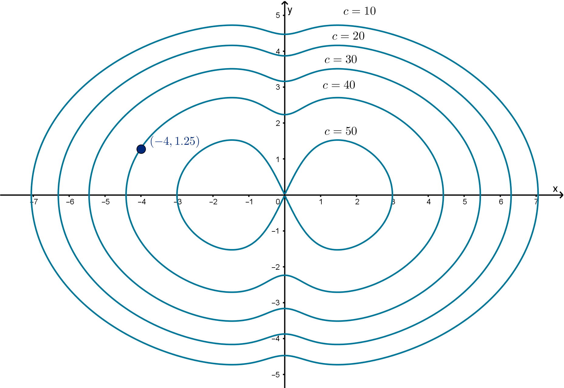
Figure: Some level curves of f (x, y )
307
Question 4.4.4
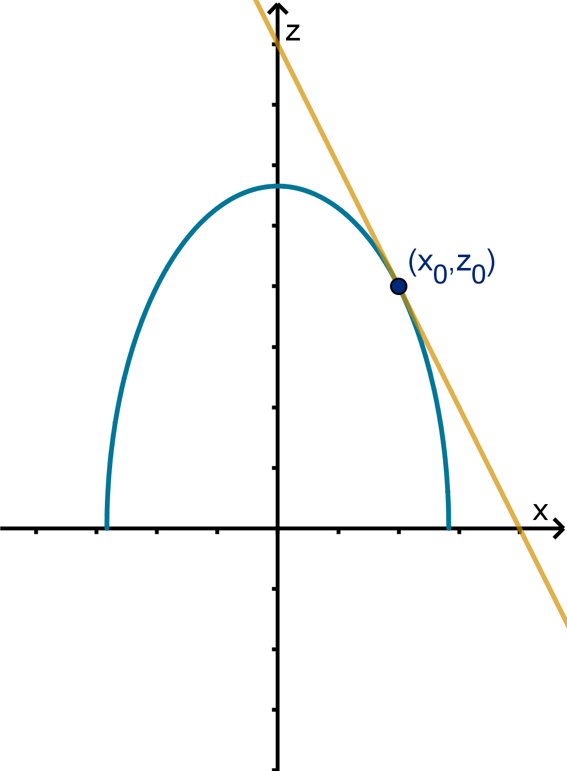
What Is the Geometric Significance of a Partial Derivative?
The partial derivative f
x
(x
0
, y
0
) is realized geometrically as the slope of
the line tangent to z = f (x, y ) at (x
0
, y
0
, z
0
) and traveling in the x
direction. Since y is held constant, this tangent line lives in y = y
0
.
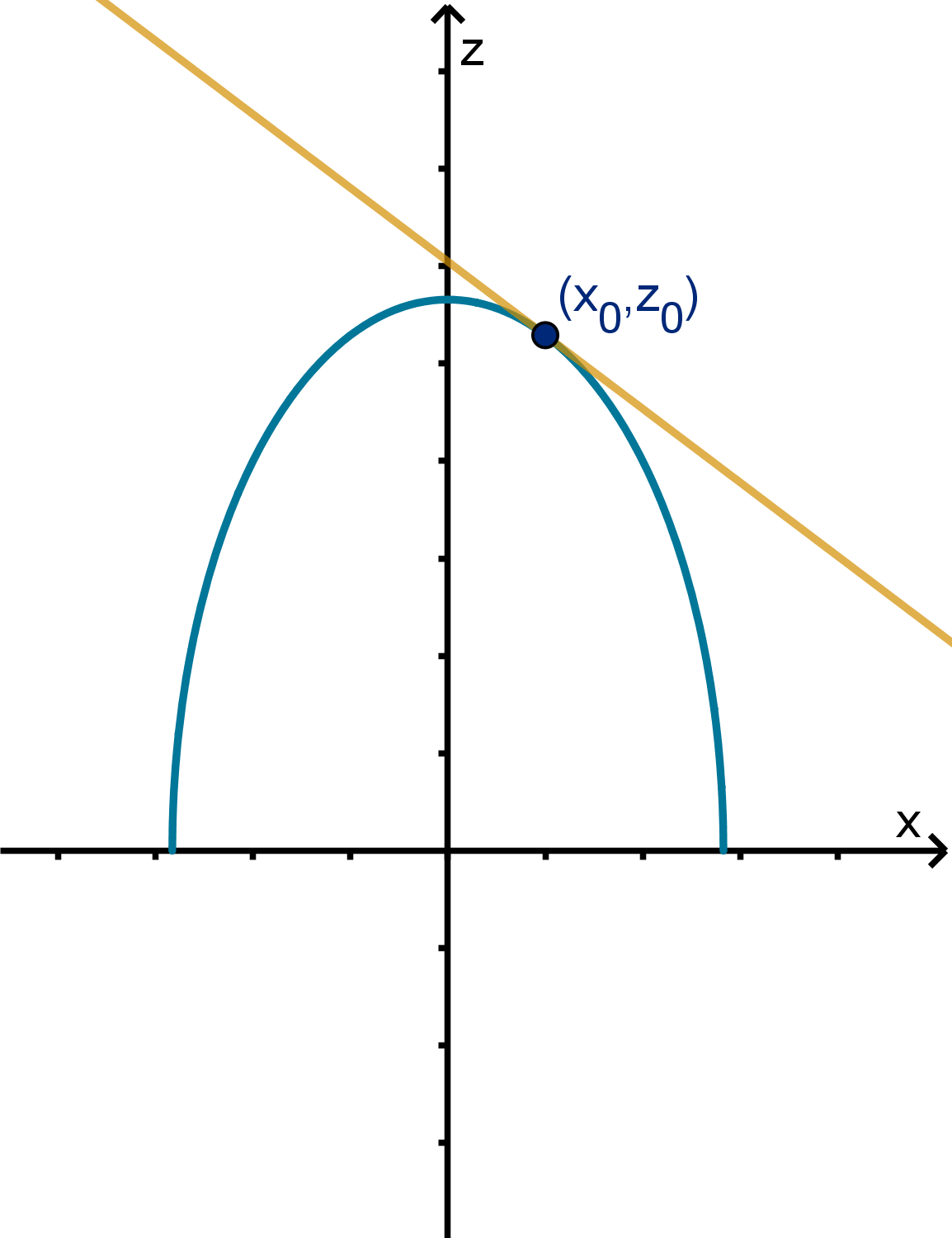
Figure: The tangent line to z = f (x, y ) in the x direction
308
Example 4.4.5
Derivative Rules and Partial Derivatives
Find f
x
for the following functions f (x, y ):
a f =
√
xy (on the domain x > 0, y > 0)
b f =
y
x
c f =
√
x + y
d f = sin (xy )
309
Question 4.4.6
What If We Have More than Two Variables?
We can also calculate partial derivatives of functions of more variables.
All variables but one are held to be constants. For example if
f (x, y, z) = x
2
− xy + cos(yz) − 5z
3
then we can calculate
∂f
∂y
:
310
Example 4.4.7
A Function of Three Variables
For an ideal gas, we have the law P =
nRT
V
, where P is pressure, n is the
number of moles of gas molecules, T is the temperature, and V is the
volume.
a Calculate
∂P
∂V
.
b Calculate
∂P
∂T
.
c (Science Question) Suppose we’re heating a sealed gas contained in
a glass container. Does
∂P
∂T
tell us how quickly the pressure is
increasing per degree of temperature increase?
311
Question 4.4.8
How Do Higher Order Derivatives Work?
Taking a partial derivative of a partial derivative gives us a higher order
partial derivative. We use the following notation.
Notation
(f
x
)
x
= f
xx
=
∂
2
f
∂x
2
We need not use the same variable each time
Notation
(f
x
)
y
= f
xy
=
∂
∂y
∂
∂x
f =
∂
2
f
∂y∂x
312
Example 4.4.9
A Higher Order Partial Derivative
If f (x, y) = sin(3x + x
2
y) calculate f
xy
.
313
Question 4.4.10
Does Differentiation Order Matter?
No. Specifically, the following is due to Clairaut:
Theorem
If f is defined on a neighborhood of (a, b) and the functions f
xy
and f
yx
are both continuous on that neighborhood, then f
xy
(a, b) = f
yx
(a, b).
This readily generalizes to larger numbers of variables, and higher order
derivatives. For example f
xyyz
= f
zyxy
.
314
Section 4.4
Summary Questions
Q1 What is the role of each variable when we compute a partial
derivative?
Q2 What does the partial derivative f
y
(a, b) mean geometrically?
Q3 Can you think of an example where the partial derivative does not
accurately model the change in a function?
Q4 What is Clairaut’s Theorem?
315
Section 4.4
Q10
In the diagram from this example, use a point on the c = 30 level set to
approximate f
y
(4, −1.25).
Figure: Some level curves of f (x, y )
316
Section 4.4
Q20
Suppose Jinteki Corporation makes widgets which is sells for $100 each.
It commands a small enough portion of the market that its production
level does not affect the demand (price) for its products. If W is the
number of widgets produced and C is their operating cost, Jinteki’s
profit is modeled by
P = 100W − C .
Since
∂P
∂W
= 100 does this mean that increasing production can be
expected to increase profit at a rate of $100 per widget?
317
Section 4.4
Q28
How many third partial derivatives does a two-variable function have?
Assuming these derivatives are continuous, which of them are equal
according to Clairaut’s theorem?
318
Section 4.5
Linear Approximations
Goals:
1 Calculate the equation of a tangent plane.
2 Rewrite the tangent plane formula as a linearization or differential.
3 Use linearizations to estimate values of a function.
4 Use a differential to estimate the error in a calculation.
Question 4.5.1
What Is a Tangent Plane?
Definition
A tangent plane at a point P = (x
0
, y
0
, z
0
) on a surface is a plane
containing the tangent lines to the surface through P.
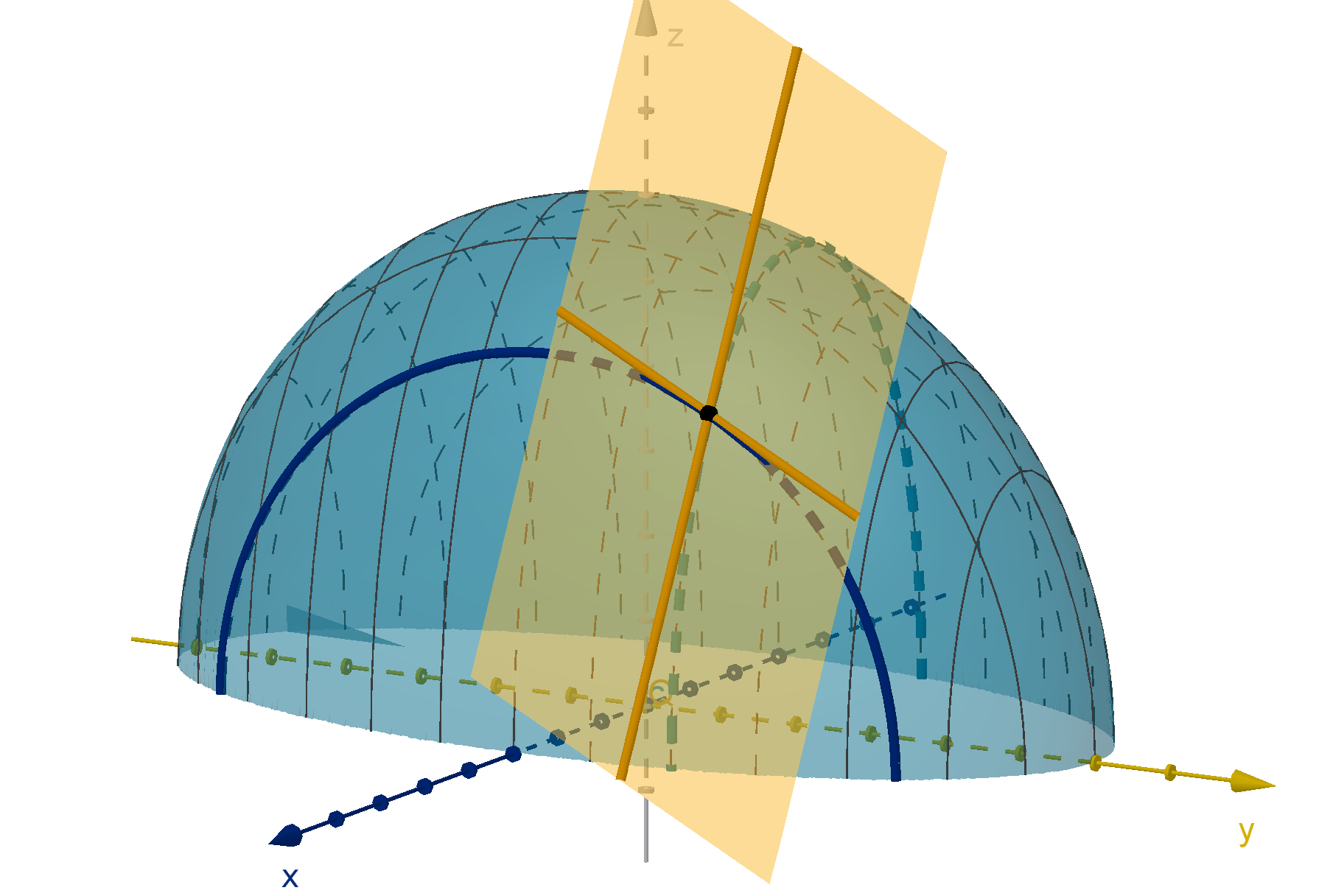
Figure: The tangent plane to z = f (x, y ) at a point
320
Question 4.5.1
What Is a Tangent Plane?
Equation
If the graph z = f (x, y ) has a tangent plane at (x
0
, y
0
), then it has the
equation:
z − z
0
= f
x
(x
0
, y
0
)(x − x
0
) + f
y
(x
0
, y
0
)(y − y
0
).
Remarks
1 This is the point-slope form of the equation of a plane. f
x
(x
0
, y
0
)
and f
y
(x
0
, y
0
) are the slopes.
2 x
0
and y
0
are numbers, so f
x
(x
0
, y
0
) and f
y
(x
0
, y
0
) are numbers. The
variables in this equation are x, y and z.
321
Question 4.5.1
What Is a Tangent Plane?
The cross sections of the tangent plane give the equation of the tangent
lines we learned in single variable calculus.
y = y
0
x = x
0
z − z
0
= f
x
(x
0
, y
0
)(x − x
0
) + 0 z − z
0
= 0 + f
y
(x
0
, y
0
)(y − y
0
)
322
Example 4.5.2
Writing the Equation of a Tangent Plane
Give an equation of the tangent plane to f (x, y) =
√
xe
y
at (4, 0)
323
Question 4.5.3
How Do We Rewrite a Tangent Plane as a Function?
Definition
If we write z as a function L(x, y), we obtain the linearization of f at
(x
0
, y
0
).
L(x, y) = f (x
0
, y
0
) + f
x
(x
0
, y
0
)(x − x
0
) + f
y
(x
0
, y
0
)(y − y
0
)
If the graph z = f (x, y ) has a tangent plane, then L(x, y ) approximates
the values of f near (x
0
, y
0
).
Notice f (x
0
, y
0
) just calculates the value of z
0
. This formula is equivalent
to the tangent plane equation after we solve for z by adding z
0
to both
sides.
324
Example 4.5.4
Approximating a Function
Use a linearization to approximate the value of
√
4.02e
0.05
.
325
Question 4.5.5
How Does Differential Notation Work in More Variables?
The differential dz measures the change in the linearization of f (x, y)
given particular changes in the inputs: dx and dy . It is a useful
shorthand when one is estimating the error in an initial computation.
Definition
For z = f (x, y), the differential or total differential dz is a function of
a point (x
0
, y
0
) and two independent variables dx and dy.
dz = f
x
(x
0
, y
0
)dx + f
y
(x
0
, y
0
)dy
=
∂z
∂x
dx +
∂z
∂y
dy
Remark
The differential formula is just the tangent plane formula with
dz = z − z
0
dx = x − x
0
dy = y − y
0
.
326
Question 4.5.5
How Does Differential Notation Work in More Variables?
An old trigonometry application is to measure the height of a pole by
standing at some distance. We then measure the angle θ of incline to the
top, as well as the distance b to the base. The height is h = b tan θ.
a If the distance to the base is 13m and the angle of incline is
π
6
, what
is the height of the pole?
b Human measurement is never perfect. If our measurement of b is off
by at most 0.1m and our measurement of θ is off by at most
π
120
, use
a differential to approximate the maximum possible error in our h.
327
Section 4.5
Summary Questions
Q1 What do you need to compute in order to write the equation of a
tangent plane to z = f (x, y ) at (x
0
, y
0
, z
0
)?
Q2 For what kinds of functions are linear approximations useful?
Q3 How are the tangent plane and the linearization related?
Q4 How is the differential defined for a two variable function? What
does each variable in the formula mean?
328
Section 4.5
Q10
Let g(x, y) =
3x
2
+4x−2
e
(y
3
)
. Write the equation of the tangent plane to
z = g (x, y ) at (0, 1).
329
Section 4.5
Q16
Show how to use an appropriate linearization to approximate
1
5.12
sin
31π
30
.
a What function f (x, y) would you linearize to make this
approximation?
b What (x
0
, y
0
) would you use to write your linearization?
c What x and y would you plug into L(x, y ) to approximate
1
5.12
sin
31π
30
?
330
Section 4.5
Q21
Boris is measuring the area of a rectangular field, so he can decide how
much grass seed to buy. According to his measurements, the field is 30m
by 50m, giving an area of 1500m
2
. If we accept that each of his
measurements has an error no larger than 0.2m, use a differential to
approximate the maximum error in his area computation.
331
Section 4.5
Q22
Suppose I decide to invest $10, 000 expecting a 6% annual rate of return
for 12 years, after which I’ll use it to purchase a house. The formula for
compound interest
P = P
0
e
rt
indicates that when I want to buy a house, I will have P = 10, 000e
0.72
.
I accept that my expected rate of return might have an error of up to
dr = 2%. Also, I may decide to buy a house up to dt = 3 years before or
after I expected.
a Write the formula for the differential dP at (r
0
, t
0
) = (0.06, 12).
b Given my assumptions, what is the maximum estimated error dP in
my initial calculation?
c What is the actual maximum error in P?
332
Section 4.5
Q24
Let f (x, y) be a function. What differential and what inputs into that
differential would you use to approximate f (5.5, 3.2) − f (4.7, 3.8).
333