Question 2.1.1
How Is the Integral Related to Geometric Area?
This region has an area of
38
3
, but
Z
8
3
f (x) dx = −
38
3
.
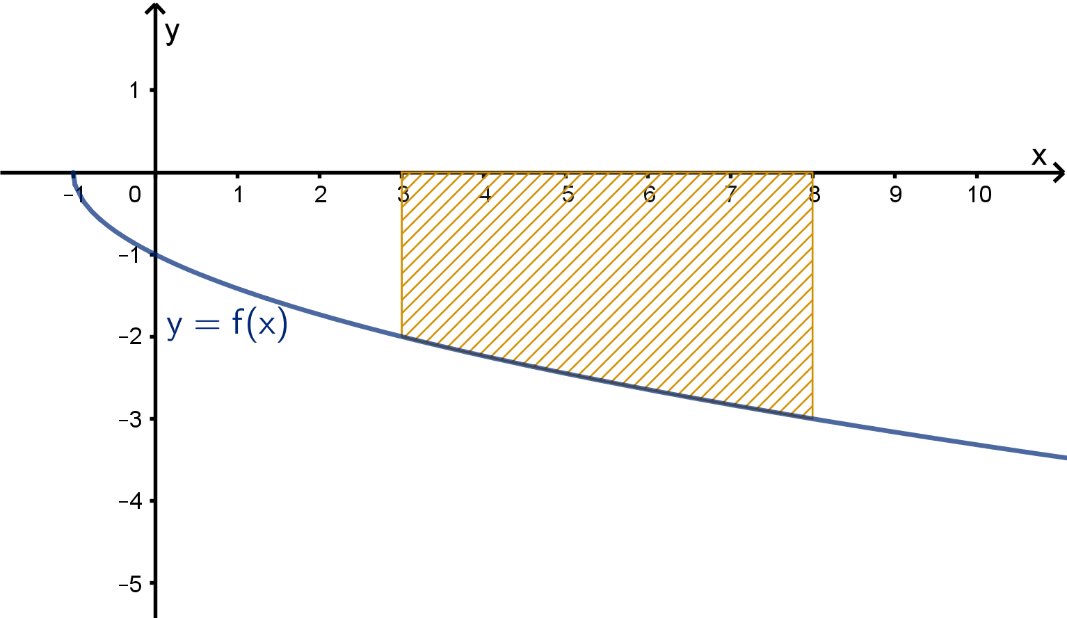
Figure: A region below the x-axis and above y = f (x)
11
Question 2.1.1
How Is the Integral Related to Geometric Area?
Why does this happen?
Definition
The integral is computed by the following limit
Z
b
a
f (x) dx = lim
∆x→0
X
i
f (x
∗
i
)∆x
When f (x) < 0, the product f (x
∗
i
)∆x computes a negative “area” for
each rectangle.
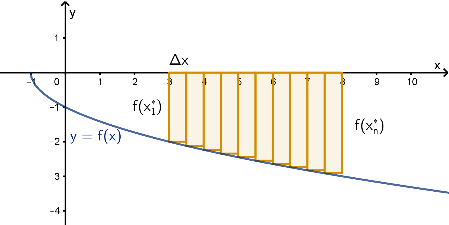
Figure: An approximation by rectangles of negative height
12
Question 2.1.2
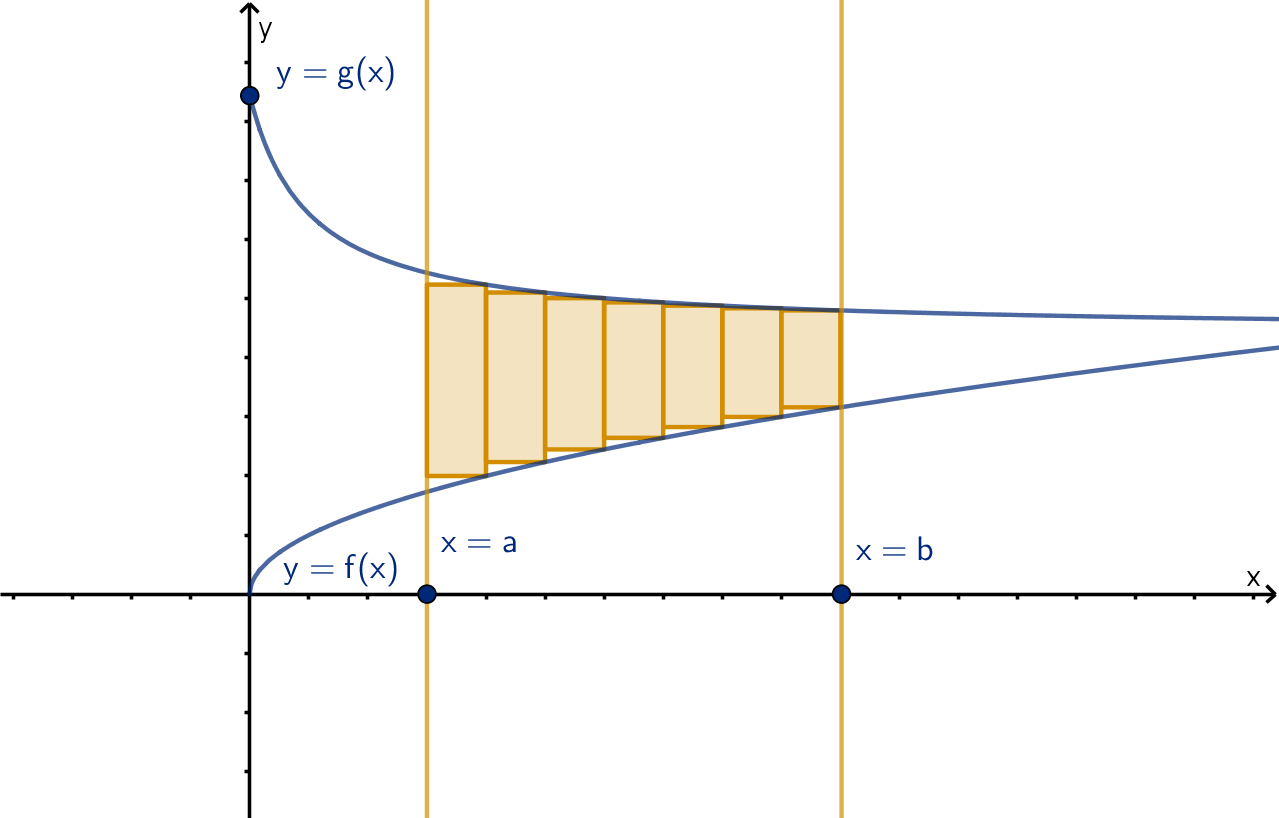
What Integral Computes the Geometric Area Between Two Graphs?
Suppose we want to know the area between the graphs y = f (x) and
y = g (x) for some interval a ≤ x ≤ b. We can approximate this by
rectangles. As the number of rectangles increases, the approximation
becomes more accurate.
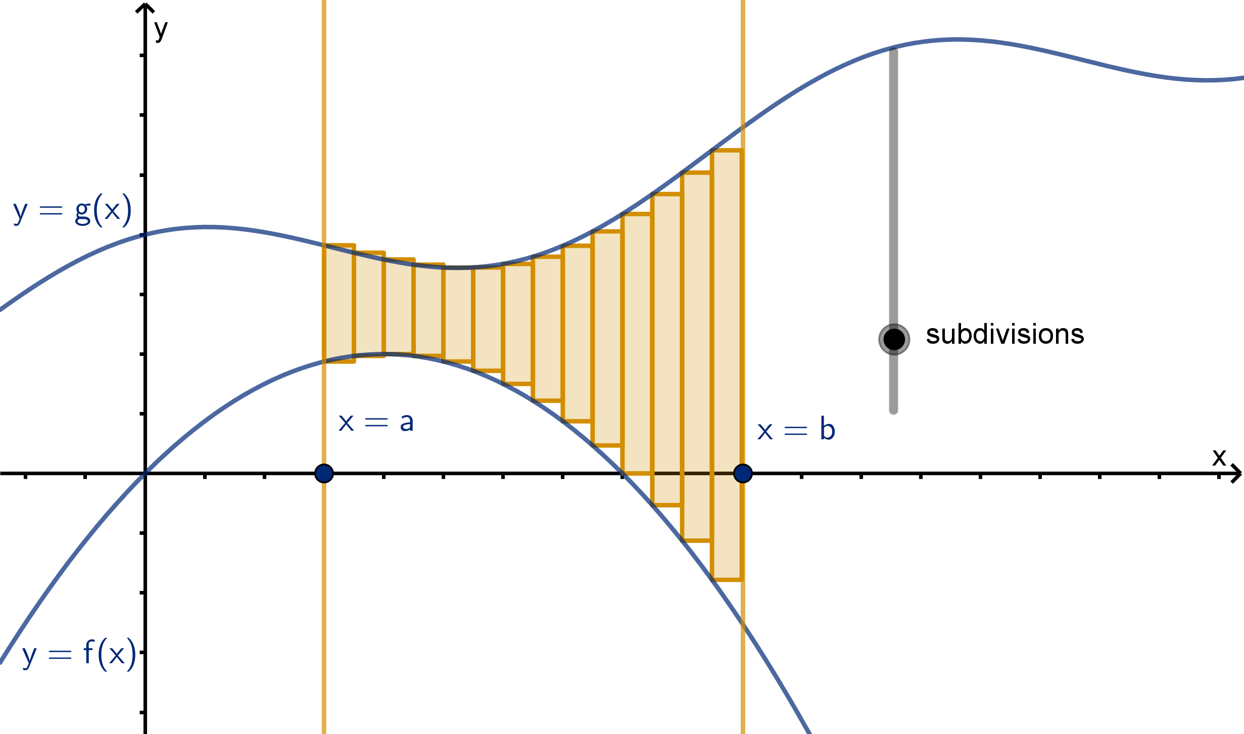
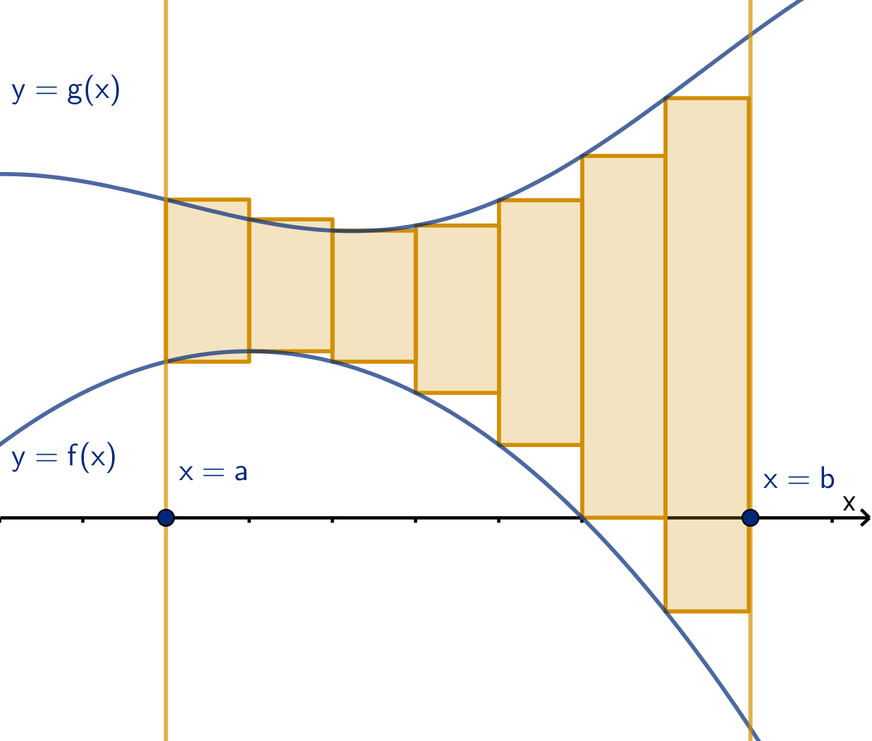
Figure: The region between y = f (x) and y = g (x), approximated by rectangles
13
Question 2.1.2
What Integral Computes the Geometric Area Between Two Graphs?
Let’s derive a formula for this rectangle approximation.
14
Question 2.1.2
What Integral Computes the Geometric Area Between Two Graphs?
Main Idea
The area above y = f (x) and below y = g(x) from x = a to x = b is
computed
Z
b
a
g(x) − f (x) dx.
15
Example 2.1.3
The Area Between Two Curves
Suppose we want to compute the area between y =
√
x and y = x −
√
x
from x = 6 to x = 12.
How do we know which graph is on top and which is on the bottom?
16
Example 2.1.3 The Area Between Two Curves
Exercise
We’ve established that at x = 9, y = x −
√
x is above y =
√
x.
Unfortunately there are infinitely many points between x = 6 and
x = 12. How can we decide which graph is on top at each of them?
1 Does the graph of y =
√
x intersect the graph of y = x −
√
x
between x = 6 and x = 12?
2 What theorem could we use to argue that if y =
√
x is ever above
y = x −
√
x then the graphs must have intersected?
17
Example 2.1.3 The Area Between Two Curves
Figure: An approximation of the area between y = x −
√
x and y =
√
x
Main Ideas
Plugging a test point into f (x) and g(x) tells us which graph is
above the other.
If the functions are continuous, then solving f (x) = g (x) computes
the only points where the graphs can change positions.
18
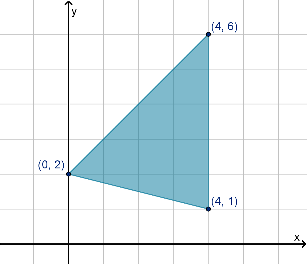
Example 2.1.4
The Area Enclosed by Two Curves
Set up an integral that computes the area enclosed between the curves
y = x
2
and y = 3 − x − x
2
.
19
Example 2.1.4
The Area Enclosed by Two Curves
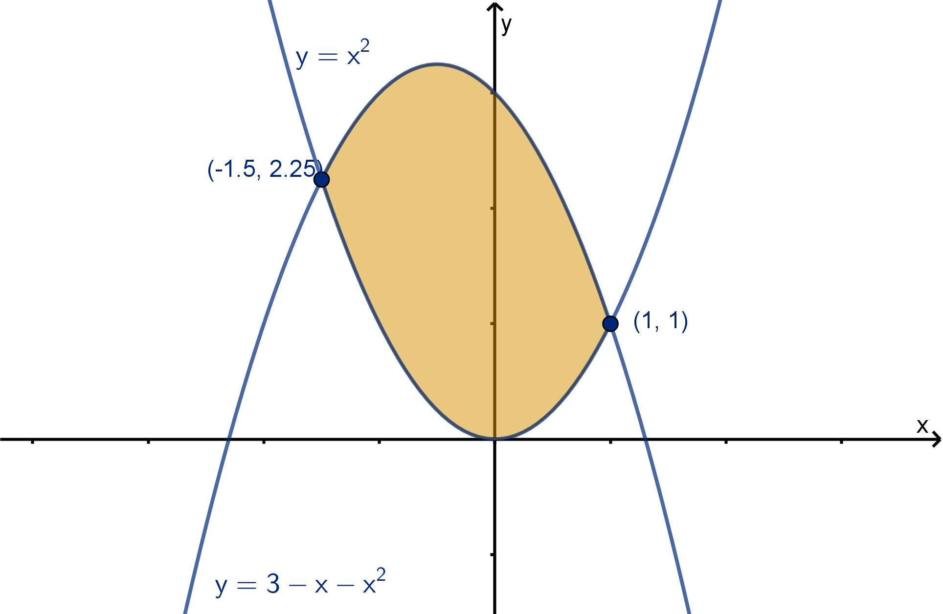
Figure: The area enclosed by two parabolas
Main Ideas
To determine the range of x values that define an enclosed region,
solve for the intersection points between the graphs.
Sketching the graphs can be a time-saver and a reality check for
your answer.
20
Example 2.1.5
The Area Enclosed by Two Curves that Intersect More than Twice
Compute the area enclosed by f (x) = x
3
− 10x and g(x) = 3x
2
.
21
Example 2.1.5
The Area Enclosed by Two Curves that Intersect More than Twice
Main Ideas
With more intersections, we must check the region between each
pair of intersections to see which graph is on top.
It can be more efficient to make a sign analysis chart.
Sketching the graphs may be more difficult. If you can do it, it will
corroborate (or correct) your calculations.
22
Example 2.1.6
A Region without a Single Top Curve
Compute the area enclosed by the curves y = 1, y =
16
x
and y = 2
√
x.
We should start by drawing this region and finding the coordinates of the
intersections.
23
Example 2.1.6
A Region without a Single Top Curve
Since the upper boundary is defined by a different function for different
values of x, one approach is to break the region into two integrals.
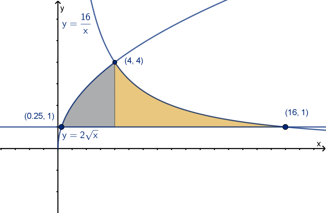
Figure: Two subregions whose areas can be expressed by integrals
24
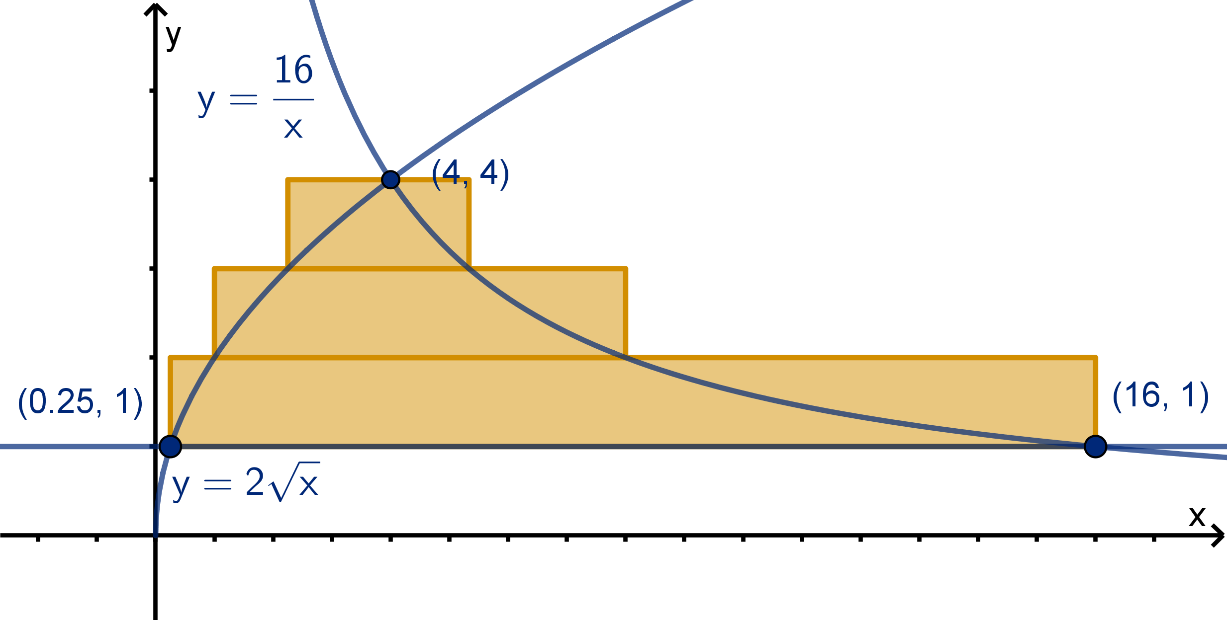
Example 2.1.6
A Region without a Single Top Curve
Instead we can approximate the region by rectangles of different widths.
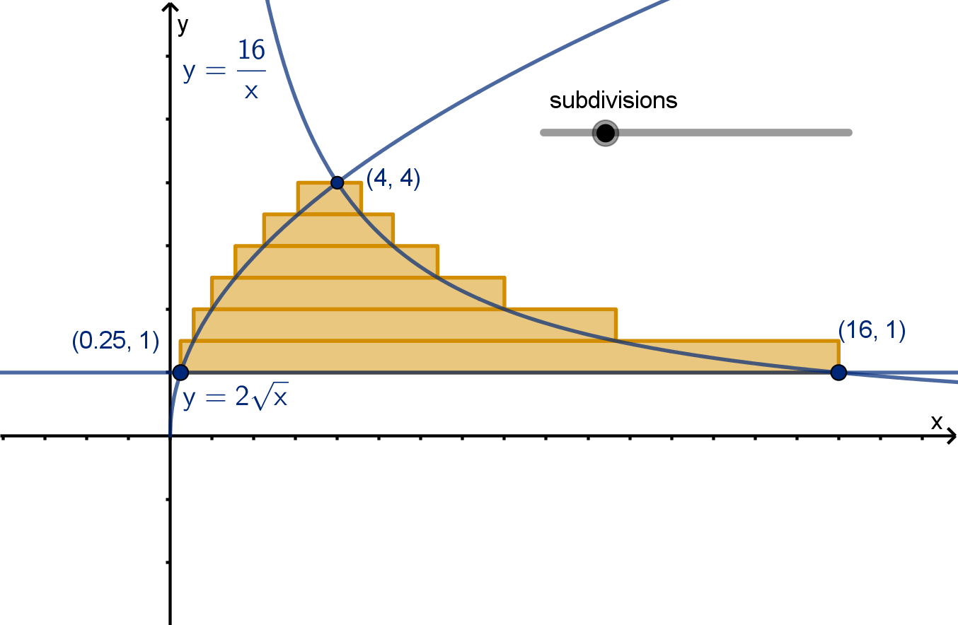
Notice the left endpoint always lies on y = 2
√
x and the right endpoint
always lies on y =
16
x
. As the height of the rectangles goes to 0, the
approximation becomes exact.
25
Example 2.1.6
A Region without a Single Top Curve
Let’s derive a formula for this rectangle approximation and compute the
exact area.
26
Example 2.1.6
A Region without a Single Top Curve
Main Idea
The area to the right of x = f
−1
(y) and to the left of x = g
−1
(y) for y
from a to b can be computed
Z
b
a
g
−1
(y) − f
−1
(y) dy .
Strategy
Changing an integral to dy may be more work than breaking it into two
or more parts. When solving an area problem, consider both methods
and use the one that seems more promising. If you run into problems
with your chosen approach, give the other method a try.
27
Section 2.1
Summary Questions
Q1 What is the geometric significance of f (x) − g(x) in the formula for
the area between two graphs?
Q2 How do we determine which curve is the top of a region and which
is the bottom? Describe the difficulties that can arise.
Q3 How do we use boundaries of the form y = g (x) and y = f (x) in an
dy-integral to compute geometric area?
Q4 When setting up a dy -integral, how can we visually identify which
graph’s function will be subtracted from which?
28
Section 2.1
Q20
Erica and Carter were asked to compute the area enclosed by y = 4x and
y = x
3
. They agree that 4x = x
3
when x = −2 and when x = 2. Erica
thinks the area is
Z
2
−2
4x − x
3
dx
Carter thinks it is
Z
2
−2
x
3
− 4x dx
a Who is correct?
b How do you think the mistake could reasonably have happened, and
how can you avoid it?
29
Section 2.1
Q20
29
Section 2.1
Q20
Main Ideas
Solve by factoring, not canceling.
Sketching the graphs can be a timesaver and a reality check for your
answer (really!)
29
Section 2.1
Q32
Suppose you are given that for all x:
f
′
(x) > 0
g
′
(x) < 0
We approximate area between y = f (x) and y = g (x) from x = a to
x = b by rectangles, letting the x
∗
i
be the right endpoints of each
subinterval. What can we say about whether the approximation will
overestimate or underestimate the true area?
30
Section 2.1
Q32
30
Section 2.2
Volumes
Goals:
1 Recognize cross sections of a solid object.
2 Write the area of each cross section as a function.
3 Compute the volume of a solid.
4 Visualize and compute the volume of a solid of revolution.
Question 2.2.1
What Is Volume?
Dimension
In mathematics, we define the dimension of an object. Dimension
measures the number of degrees of freedom available to a point traveling
in the object.
Example
1 A plane is two dimensional. You can travel left/right or up/down.
2 A circle is one dimensional. You can only travel
clockwise/counterclockwise.
3 A point is zero dimensional. There is nowhere to travel within it.
32
Question 2.2.1
What Is Volume?
We measure objects of different dimensions differently. In all cases,
measuring is counting how many units of measurement fit inside the
object.
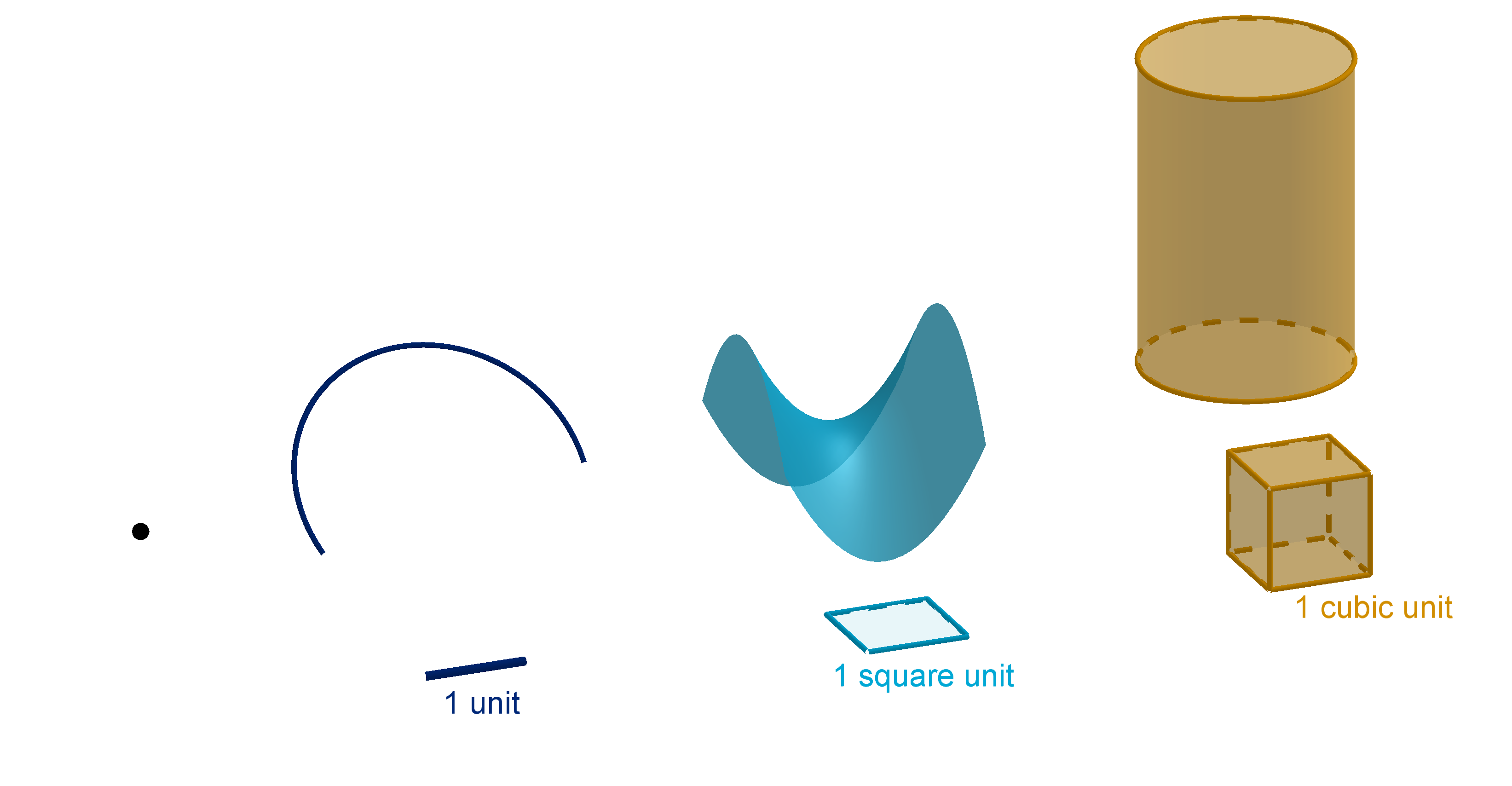
Figure: Objects of several dimensions and their units of measurement
33
Question 2.2.1
What Is Volume?
We use different names to describe objects and their measurements in
different dimensions:
Dimension Names Measurement
0 point none
1 line, circle, curve length
2 square, polygon, disc, sphere, surface area
3 cube, polyhedron, ball, solid volume
Vocabulary Check
It doesn’t make sense to talk about the volume of a surface. No unit
cubes will fit inside it.
Similarly it doesn’t make sense to talk about the area of a solid. Infinitely
many unit squares will fit in any solid. However, solids have boundary
surfaces, and we do sometimes measure their areas.
34
Question 2.2.1
What Is Volume?
Formula for Volume of a Prism
volume = area of base × height
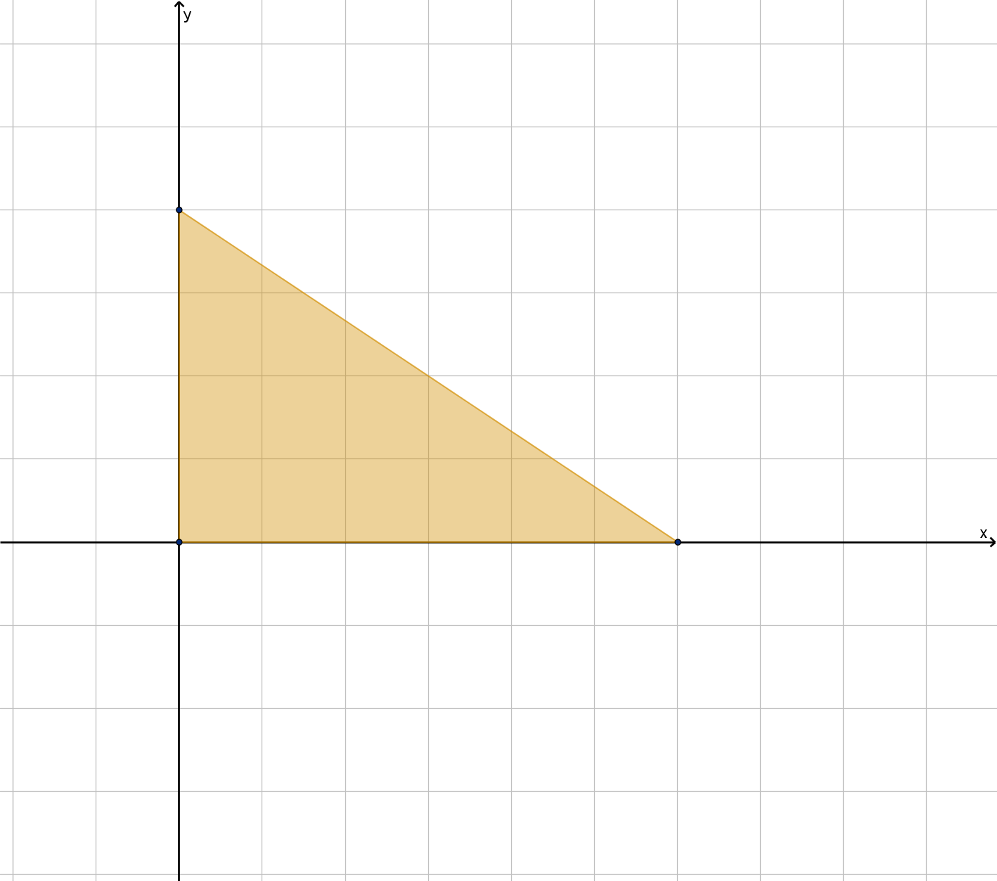
Figure: A prism divided into unit cubes and its base divided into unit squares.
35
Question 2.2.1
What Is Volume?
Remark
Our motivation for studying solids is not to solve geometry problems.
Recall that the definite integral allowed us to express total change as an
area:
total change = rate of change ×time
f (b) −f (a) =
Z
b
a
f
′
(t) dt
This allowed us to use our geometric intuition of areas to better
understand rates of change. Similarly, volume will allow us to use
geometry understand different types of rates later on.
36
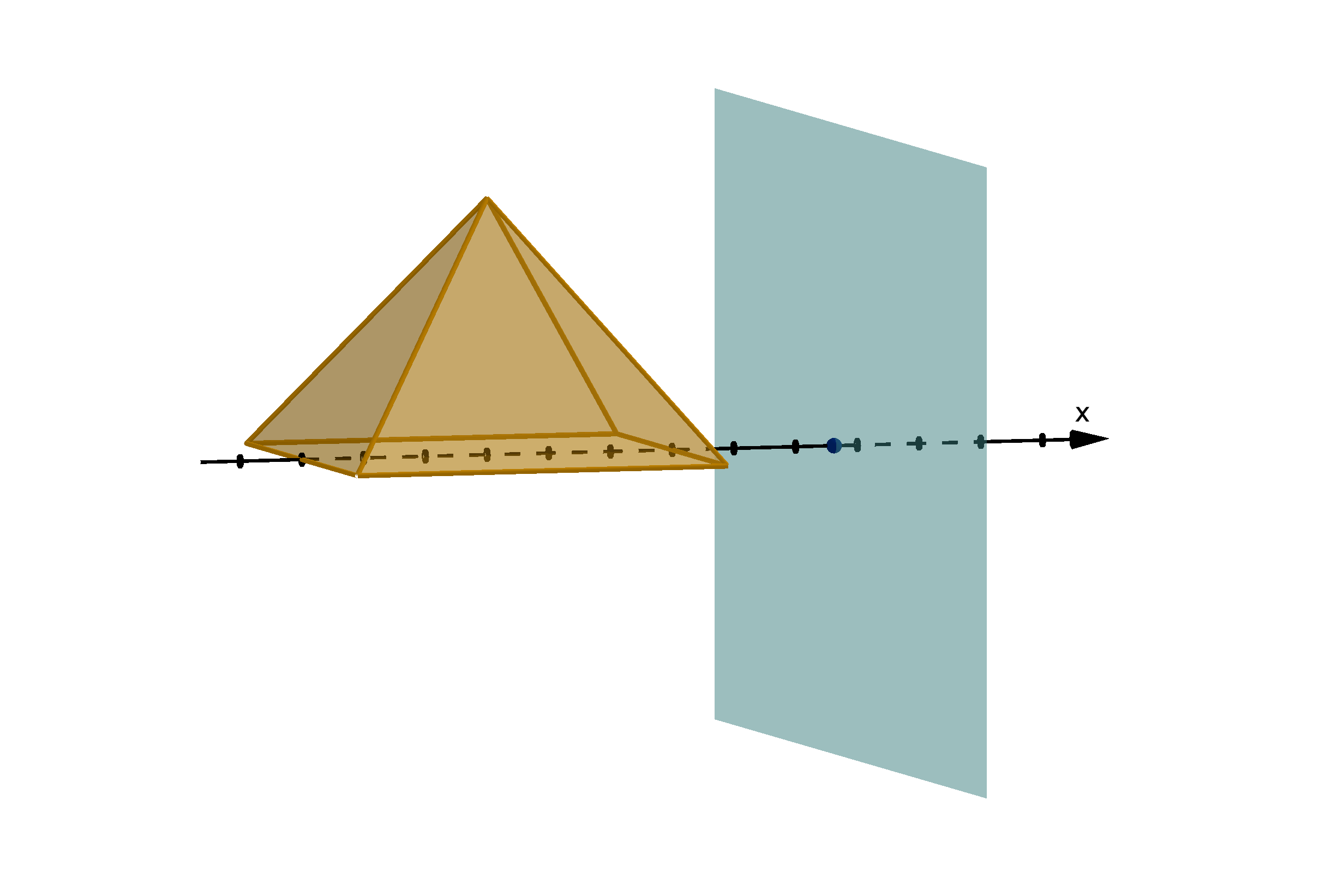
Question 2.2.2
How Do We Visualize 3-Dimensional Solids?
Definition
A cross section of a solid object is its intersection with some transversal
plane.
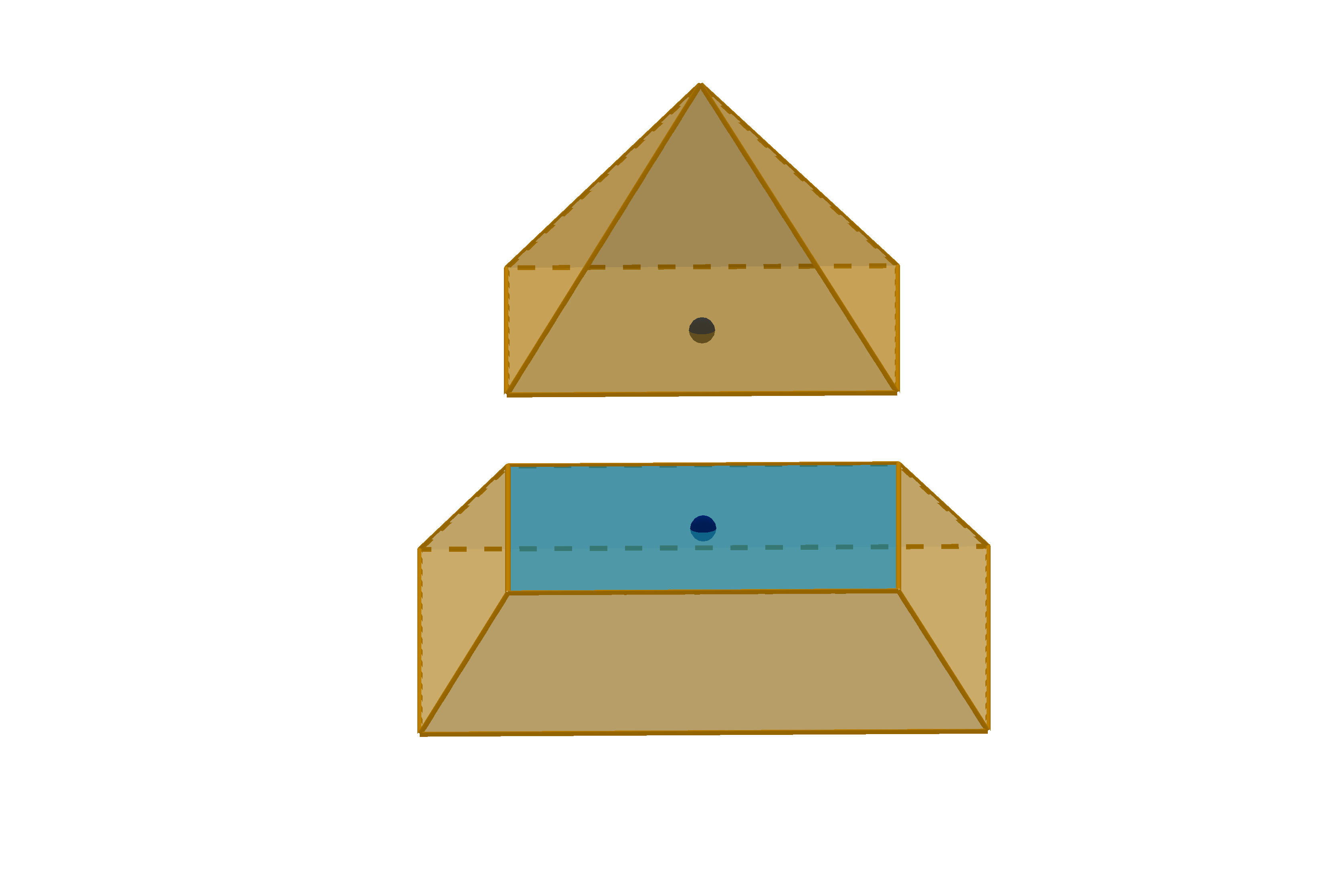
Figure: A cross section of a pyramid
37
Question 2.2.2
How Do We Visualize 3-Dimensional Solids?
A solid can be reassembled from its cross sections. This is valuable
because cross sections are two-dimensional, making them easier to draw
or visualize.
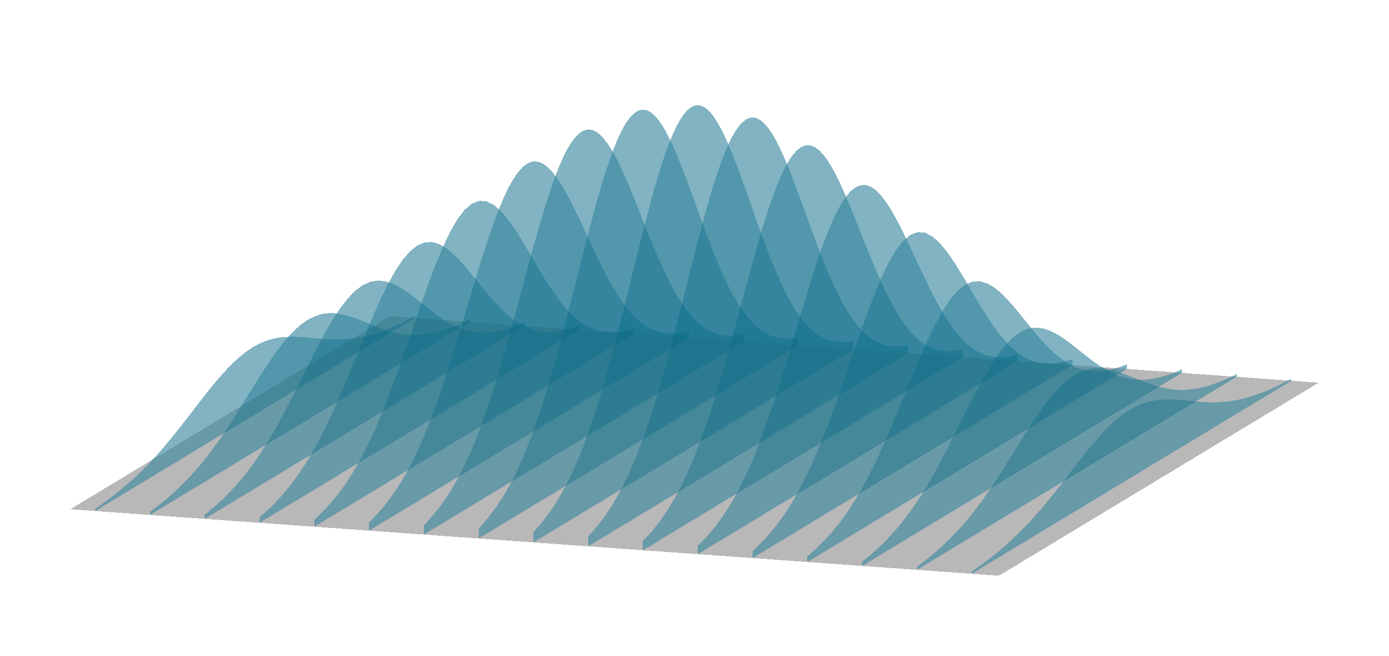
Figure: A set of parallel cross sections of a solid
38
Question 2.2.3
How Can We Approximate or Compute the Volume of a Non-Prism Solid?
Suppose we want to find the volume of a pyramid. Different square units
of the base have a different number of cubic units above them. Thus we
need a more robust approach than counting cubes.
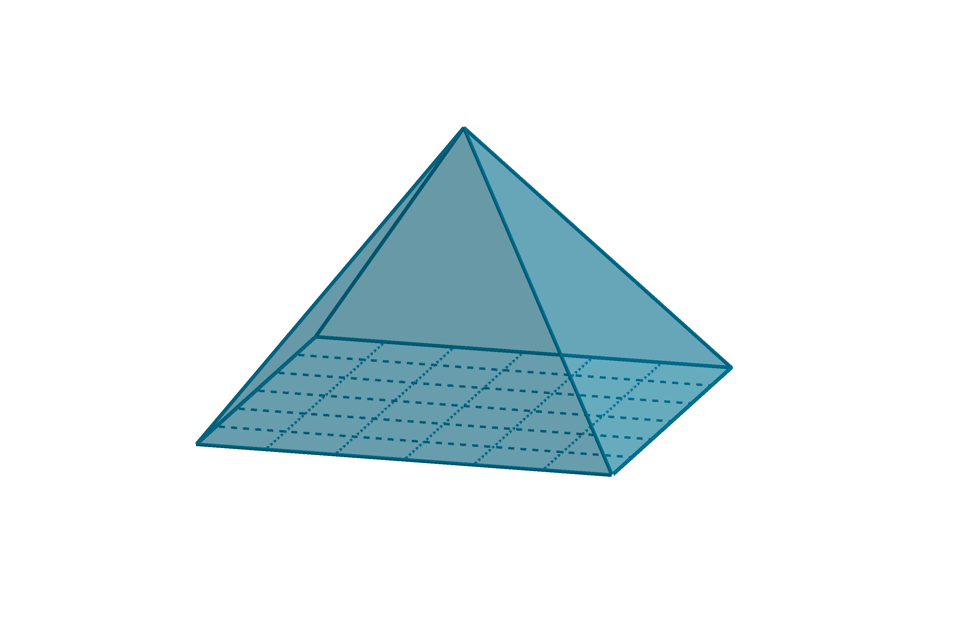
Figure: A pyramid with its base divided into unit squares
39
Question 2.2.3
How Can We Approximate or Compute the Volume of a Non-Prism Solid?
We will approximate the pyramid by prisms, whose bases are cross
sections.
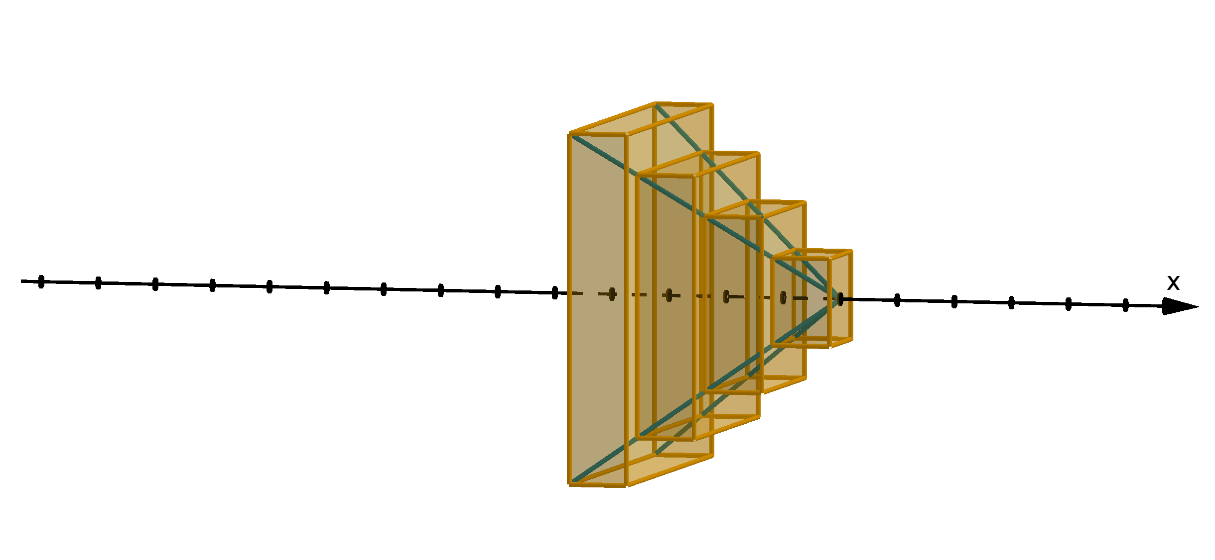
Figure: A pyramid approximated by prisms
40
Question 2.2.3
How Can We Approximate or Compute the Volume of a Non-Prism Solid?
Theorem
If the cross section of a solid, perpendicular to the x-axis, has area A(x)
at each x, then the volume of the solid is
Z
b
a
A(x) dx
where a and b are the values of x at the bottom and top of the solid.
41
Example 2.2.4
A Solid with Its Cross-Sections Given
Suppose a solid S extends from x = 2 to x = 6 and the cross section at
each x is a right triangle of height
1
x
and base x
2
. Compute the volume
of S.
42
Example 2.2.5
A Solid Obtained by Rotation
Suppose the region under the graph y =
5
x+1
from x = 1 to x = 4 is
rotated around the x-axis. Compute the volume of the resulting solid.
43
Example 2.2.5
A Solid Obtained by Rotation
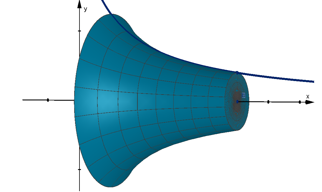
Figure: The solid obtained by rotating the region under y =
5
x+1
about the
x-axis
Main Idea
When the region under a graph y = f (x) is rotated around the x-axis,
the cross sections are discs of radius f (x). Their areas are π[f (x)]
2
.
44
Example 2.2.6
A Solid Defined by Its Base
Suppose we have a solid S with the following properties:
The base of S is the region enclosed by y = 0 and y = 4x − x
2
.
The cross-sections of S perpendicular to the x-axis are trapezoids
which have one base in the base of S, another base twice as long,
and whose heights are 6 units.
Compute the volume of S.
45
Example 2.2.6
A Solid Defined by Its Base
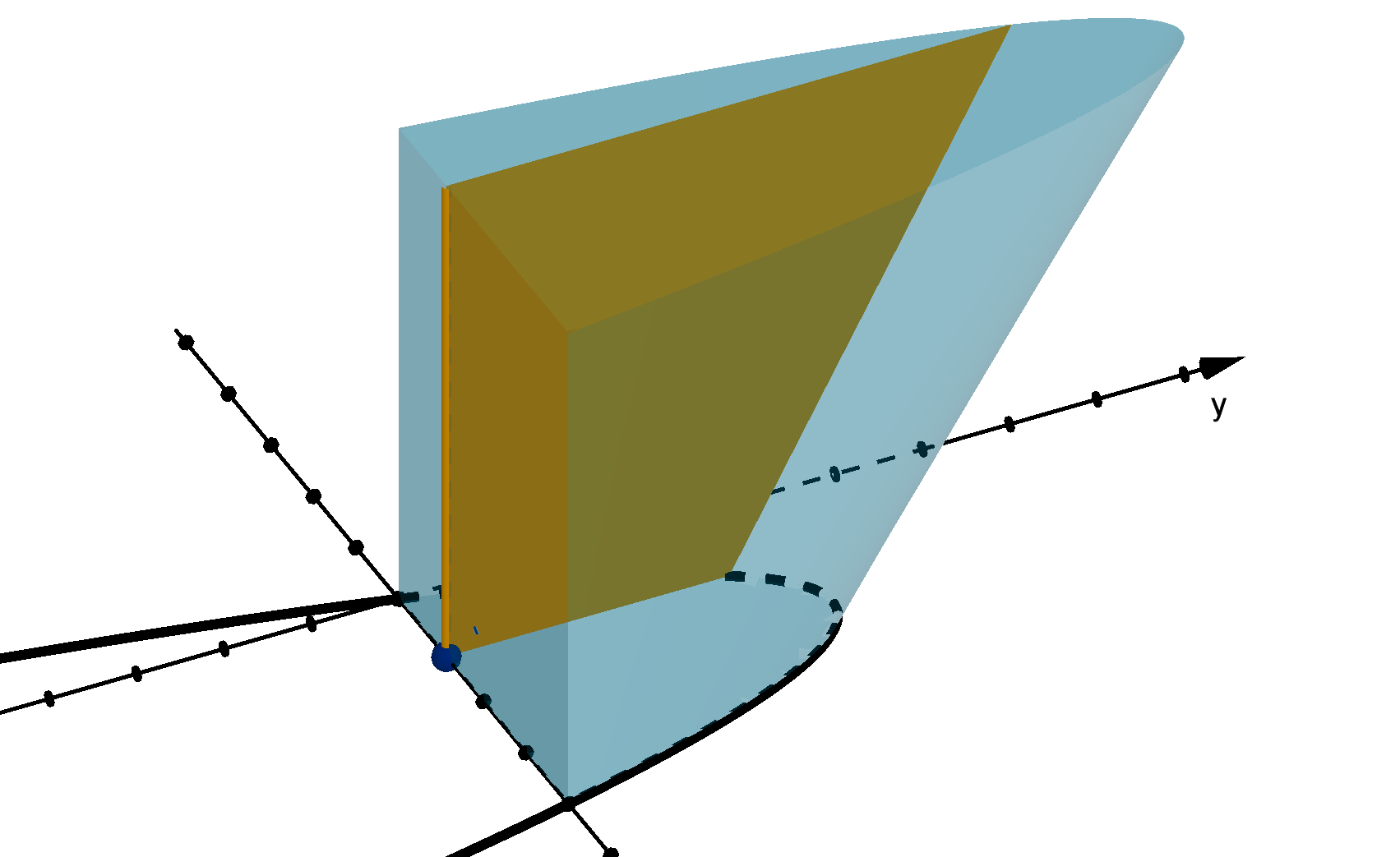
Figure: A solid with base between two graphs and trapezoidal cross-sections
Main Idea
The cross section of the base of a solid is a segment. If we know what
role this segment plays in the cross section of the solid, we can use the
expression for the length of this segment to derive an expression for A(x).
46
Example 2.2.7
A Solid Described by Measurements
Compute the volume of a pyramid with a square base of side length s
and a height of h.
47
Section 2.2
Summary Questions
Q1 Describe how a cross section of a solid is produced.
Q2 What is the significance of the function A(x) in the formula for the
volume of a solid?
Q3 What shapes do we use to approximate the volume of a solid? Why
do we choose that shape?
Q4 When we rotate the region under y = f (x) around the x axis, how
do we compute the area of each cross-section?
48
Section 2.2
Q10
Describe or draw the cross sections of the pyramid below when it is cut
by planes parallel to the one pictured.
49
Section 2.2
Q26
Compute the volume of a solid whose base is the region enclosed by
y =
√
x and y =
x
2
and whose cross sections, perpendicular to the x-axis
are squares.
50
Section 2.2
Q26
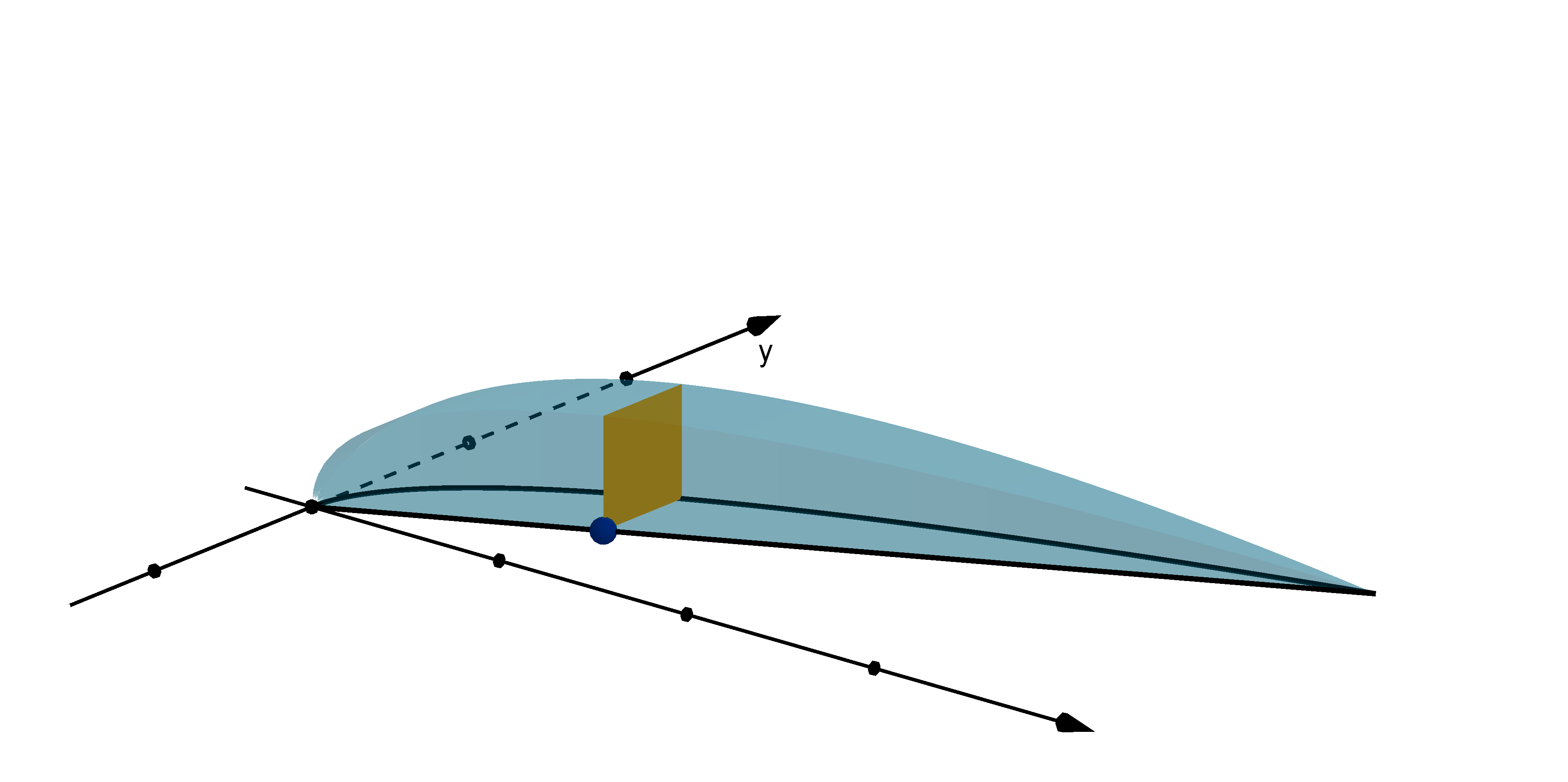
Figure: A solid with square cross sections
50
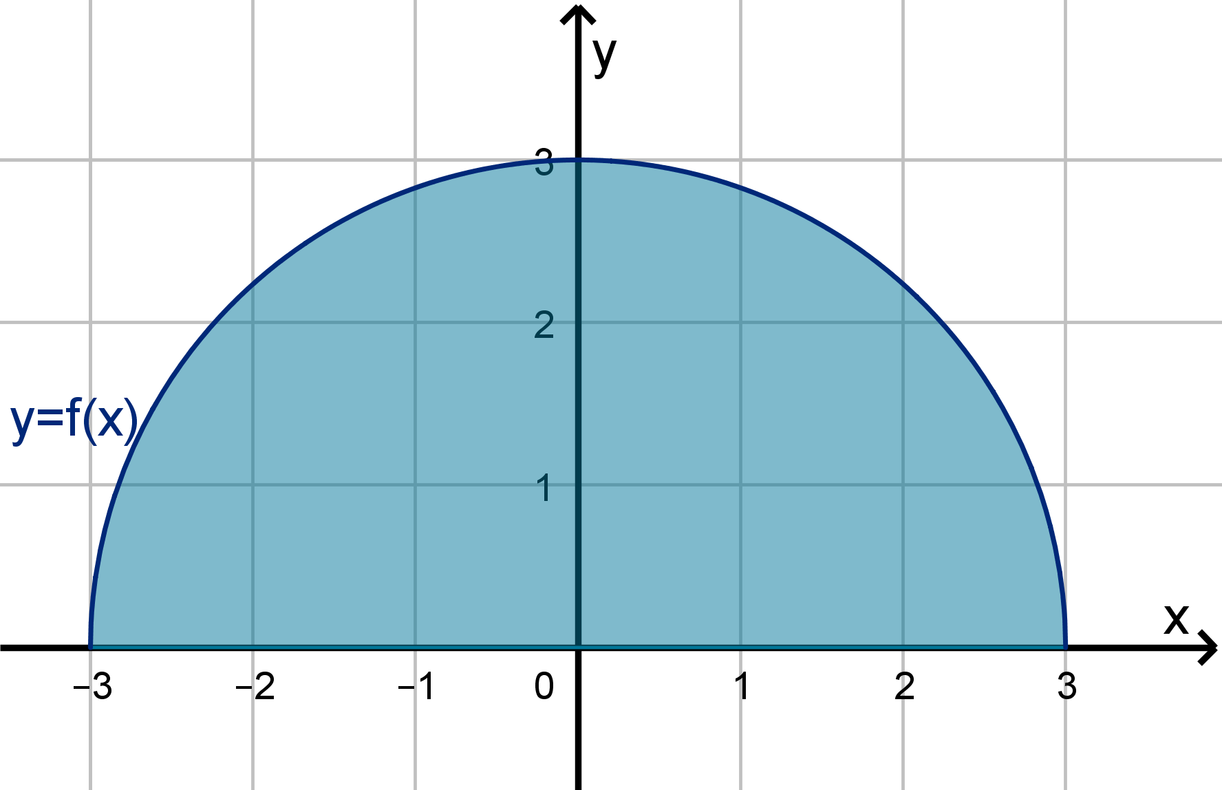
Section 2.2
Q22
Consider the semidisk of radius 3 below:
a Write a function y = f (x) that defines the boundary of this
semidisk.
b Suppose this semidisk is rotated around the x-axis. Describe the
resulting solid.
c Compute A(x), the area of the cross section at each value of x.
d Write and evaluate an integral that computes the volume the solid
of rotation.
51
Section 2.2
Q30
Consider the solid obtained by rotating the triangle below around the
x-axis.
a Describe the shape of the cross sections. Which measurements of
this shape depend on x?
b Compute a formula for A(x), the area of the cross section at each
value of x.
c Compute the volume of the solid.
52
Section 2.3
Integration by Parts
Goals:
1 Use the integration by parts formula to find anti-derivatives and
definite integrals.
2 Choose appropriate decompositions for integrating by parts.
3 Recognize when applying the formula multiple times will be fruitful.
Question 2.3.1
How Do We Compute an Anti-Derivative of a Product of Two Functions?
We reversed the chain rule (which computes derivatives) to compute
anti-derivatives of certain functions. This method is called
u-substitution.
Example
Compute the integral:
Z
3
0
xe
x
2
dx
54
Question 2.3.1
How Do We Compute an Anti-Derivative of a Product of Two Functions?
Main Idea
u-substitution is extremely fragile. Our example relies on the fact that the
factor x is a constant multiple of the derivative of the inner function, x
2
.
55
Question 2.3.1
How Do We Compute an Anti-Derivative of a Product of Two Functions?
There is another differentiation rule that produces products.
Reminder
The Product Rule states that if f (x) and g(x) are differentiable, then
[f (x)g(x)]
′
= f
′
(x)g(x) + g
′
(x)f (x).
Example
Compute
Z
x
2
cos x + 2x sin x dx
If anything, this is more fragile than u-substitution. It requires a sum of
compatible products.
56
Question 2.3.1
How Do We Compute an Anti-Derivative of a Product of Two Functions?
How can we make the formula [f (x)g (x)]
′
= f
′
(x)g(x) + g
′
(x)f (x) more
useful?
57
Question 2.3.1
How Do We Compute an Anti-Derivative of a Product of Two Functions?
This method is called integration by parts. Here is the formal
statement.
Theorem
Suppose an integral can be written
Z
u dv where
u is a function (more precisely u(x)),
and dv is a differential (more precisely v
′
(x)dx).
We can apply the following formula:
Z
u dv = uv −
Z
v du
58
Example 2.3.2
Computing an Anti-derivative Using Integration by Parts
Compute
Z
xe
x
dx.
59
Question 2.3.3
How Do We Choose u and dv ?
What would happen if we again solved
Z
xe
x
dx by parts, but set
u = e
x
dv = x dx?
60
Question 2.3.3
How Do We Choose u and dv ?
In integration by parts, u is going to be differentiated. This usually
makes functions simpler if anything. dv is going to be integrated. This
could make
Z
v du difficult to compute.
I.L.A.T.E.
When deciding which factor of a product should be u and which should
be dv, put them into the chart below.
Inverse
functions
Logarithms
Algebraic
expressions
(polyniomials)
Trig
functions
Exponential
functions
better u’s better dv’s
61
Question 2.3.3
How Do We Choose u and dv ?
Let’s apply I.L.A.T.E to the following products:
1
Z
x
5
ln x dx
2
Z
x sin x dx
3
Z
x
2
tan
−1
(x) dx
62
Example 2.3.4
Using Integration by Parts More than Once
Compute
Z
π
0
x
2
cos x dx
63
Example 2.3.4
Using Integration by Parts More than Once
Change of Variables?
Notice that despite defining functions u and v , we continue to work in
terms of the variable x. Contrast this with u-substitution where the
variable x can be completely eliminated in a definite integral. That
approach isn’t possible here. We’d have to write v as a function of u.
This would be complicated or impossible.
64
Example 2.3.5
Using Integration by Parts to Produce an Equation
Compute
Z
e
2x
cos x dx
65
Example 2.3.5
Using Integration by Parts to Produce an Equation
Main Idea
The success of integration by parts depends on the
Z
v du term.
Is
Z
v du still a product?
Integrate it.
You are done.
Can you apply a u-sub?
Use u-sub.
You are done.
How does
Z
v du compare
to the orginal integrand?
Apply integration by
parts again.
Use another
approach.
Write an equation
and solve.
no
yes
yes
no
simpler
similar
more
complicated
constant multiple
66
Section 2.3
Summary Questions
Q1 What type of integrands are good candidates for integration by
parts?
Q3 How is u handled differently in integration by parts than in
u-substitution?
Q5 How is the acronym I.L.A.T.E. used?
Q7 Under what conditions would we want to apply integration by parts
more than once?
67
Section 2.3
Q6
Which of the following can be integrated using u-substitution?
R
e
x
dx
R
xe
x
dx
R
x
2
e
x
dx
R
x
3
e
x
dx
R
e
x
2
dx
R
xe
x
2
dx
R
x
2
e
x
2
dx
R
x
3
e
x
2
dx
R
e
x
3
dx
R
xe
x
3
dx
R
x
2
e
x
3
dx
R
x
3
e
x
3
dx
R
e
x
4
dx
R
xe
x
4
dx
R
x
2
e
x
4
dx
R
x
3
e
x
4
dx
68
Section 2.3
Q10
We can write
Z
ln x dx as a product:
Z
(1)(ln x) dx.
a How does I.L.A.T.E. suggest we proceed?
b Use integration by parts to compute the antiderivative.
69
Section 2.3
Q10
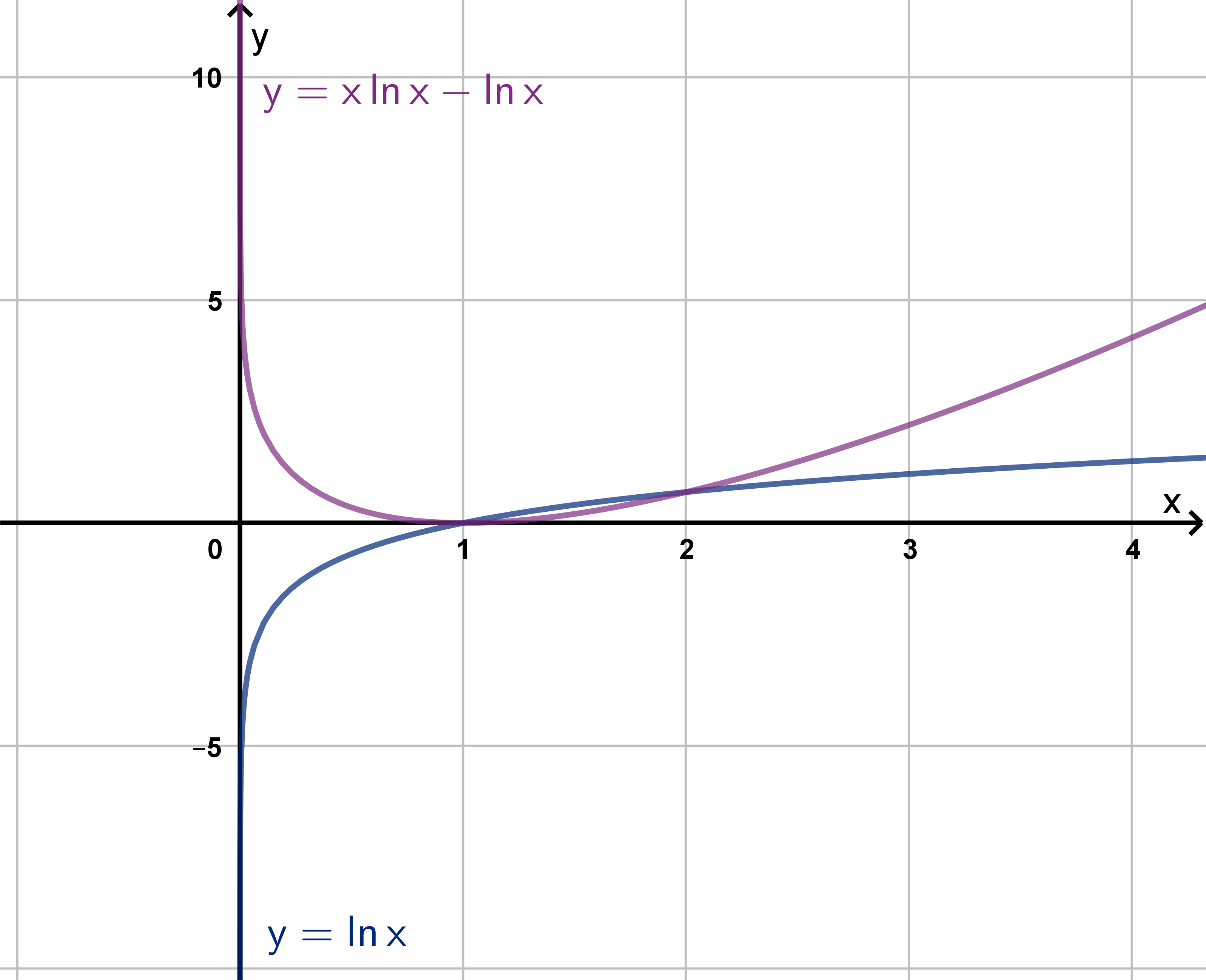
Figure: y = ln x and its antiderivative
69
Section 2.4
Approximate Integration
Goals:
1 Use several methods to approximate definite integrals.
2 Assess the accuracy of an approximation.
3 Approximate integrals given incomplete information.
Question 2.4.1
What x
∗
i
Can We Use when Approximating an Integral?
Recall the following
Definition
The definite integral is given by the formula
Z
b
a
f (x) dx = lim
∆x→0
n
X
i=1
f (x
∗
i
)∆x
where ∆x are the lengths of the subintervals of [a, b], and x
∗
i
is a number
in the i
th
subinterval.
Without the limit (which is difficult or impossible to compute anyway)
the sums on the right are approximations of the integral. Once we
choose an x
∗
i
for each i, we can evaluate this approximation.
71
Question 2.4.1
What x
∗
i
Can We Use when Approximating an Integral?
The simplest idea is to just use the left endpoint of each subinterval as
x
∗
i
.
Notation
The notation L
n
refers to the
approximation of
Z
b
a
f (x) dx by n
rectangles,
n
X
i=1
f (x
∗
i
)∆x,
where the x
∗
i
are the left endpoints of
each subinterval.
Similarly R
n
refers to the approximation
using the right endpoints for x
∗
i
.
ggb/intapproximationsln.png
L
4
approximation
72
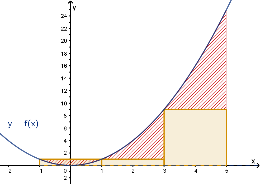
Example 2.4.2
Computing an L
n
Approximation
a Compute an L
3
approximation of
Z
5
−1
x
2
dx.
b Does L
3
over or underestimate the actual value of
Z
5
−1
x
2
dx?
73
Example 2.4.2
Computing an L
n
Approximation
74
Question 2.4.3
How Accurate is an L
n
or R
n
Approximation?
An approximation is much more useful, if we have some idea of how
accurate (or inaccurate) it might be. The way we quantify this
inaccuracy is error.
Definitions
The error in an approximation is given by
error = approximated value − actual value
In a real world approximation, we do not know the exact error (why?).
We will settle for putting a bound on error. This is a number N such
that we are sure that
|error| ≤ N.
75
Question 2.4.3
How Accurate is an L
n
or R
n
Approximation?
Determining error bounds can be difficult. Here are some questions to
ask.
1 In what circumstances is the approximation exact?
2 What property or measurement seems to correspond to the amount
of error?
3 Is there a “worst case scenario” associated to that property or
measurement?
76
Question 2.4.3 How Accurate is an L
n
or R
n
Approximation?
Exercise
a Draw a function for which L
n
is always an overestimate.
b Draw a function for which L
n
is always an underestimate.
c What has to be true of a function for L
n
to always be exact?
d What familiar calculus measurement appears to measure whether
you are in the situations you described in a - c ?
77
Question 2.4.3 How Accurate is an L
n
or R
n
Approximation?
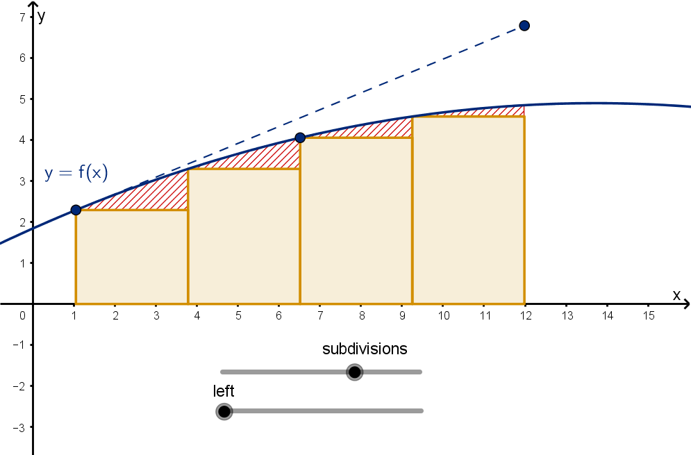
Figure: The error of an L
n
approximation
78
Question 2.4.3 How Accurate is an L
n
or R
n
Approximation?
Let’s use the results of the exercise to formulate an error bound for L
n
.
79
Question 2.4.3 How Accurate is an L
n
or R
n
Approximation?
Our result can be stated as a theorem:
Theorem
If E
L
and E
R
are the errors in an L
n
and R
n
approximations of
Z
b
a
f (x) dx and |f
′
(x)| ≤ S on [a, b] then
|E
L
| ≤
S(b − a)
2
2n
and |E
R
| ≤
S(b − a)
2
2n
80
Example 2.4.4
Computing an E
L
Bound
Suppose we want to understand the error of an L
n
approximation of
Z
16
1
√
x dx.
a What bounds can we put on |f
′
(x)| for our error calculation?
b What bound can we put on the error of the L
5
approximation?
c What n would we need in order to guarantee that the L
n
approximation has error at most
1
100
.
d What problem would result, if we tried to bound the error of an L
n
approximation of
Z
16
0
√
x dx? How might you resolve this?
81
Example 2.4.4
Computing an E
L
Bound
Suppose we want to understand the error of an L
n
approximation of
Z
16
1
√
x dx.
a What bounds can we put on |f
′
(x)| for our error calculation?
81
Example 2.4.4
Computing an E
L
Bound
Suppose we want to understand the error of an L
n
approximation of
Z
16
1
√
x dx.
b What bound can we put on the error of the L
5
approximation?
81
Example 2.4.4
Computing an E
L
Bound
Suppose we want to understand the error of an L
n
approximation of
Z
16
1
√
x dx.
c What n would we need in order to guarantee that the L
n
approximation has error at most
1
100
.
81
Example 2.4.4
Computing an E
L
Bound
Suppose we want to understand the error of an L
n
approximation of
Z
16
1
√
x dx.
d What problem would result, if we tried to bound the error of an L
n
approximation of
Z
16
0
√
x dx? How might you resolve this?
81
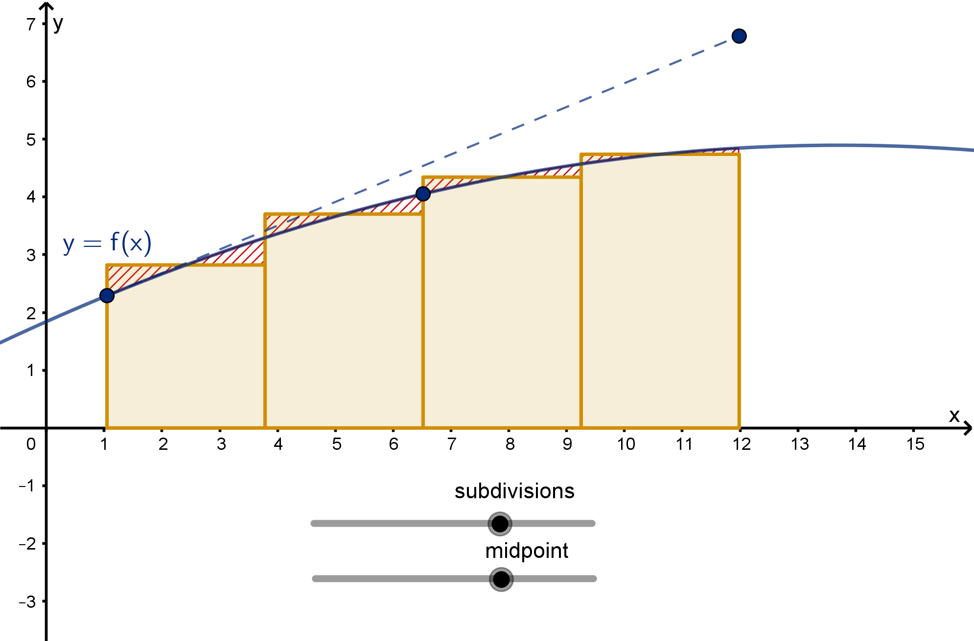
Question 2.4.5
How Can We Make our Approximation Less Sensitive to Slope?
L
n
and R
n
have large errors when function is increasing or decreasing
rapidly. We’ll examine two approximations that are more resilient. The
first is the midpoint approximation.
Notation
The M
n
approximation of
Z
b
a
f (x) dx is
calculated by summing:
n
X
i=1
f (x
∗
i
)∆x
where the x
∗
i
are the midpoints of each
subinterval.
ggb/intapproximationsmd.png
M
4
82
Question 2.4.5
How Can We Make our Approximation Less Sensitive to Slope?
Our final approximation abandons rectangles entirely. Using trapezoids
instead allows for shapes that reflect the value of the function at both
the right and left endpoint.
Notation
The T
n
approximation of
Z
b
a
f (x) dx is
calculated by summing:
n
X
i=1
1
2
(f (x
i
) + f (x
i+1
))∆x
where x
i
and x
i+1
and the two
endpoints of the i
th
subinterval.
T
n
can also be calculated as
1
2
(L
n
+ R
n
).
ggb/intapproximationstrap.png
T
4
83
Example 2.4.6
A Midpoint Approximation
Calculate the M
3
approximation of
Z
5
−1
x
2
dx.
84
Example 2.4.7
A Trapezoid Approximation Using a Table of Values
Suppose we have the following table of values for a function f (x)
x 0 2 4 6 8 10 12 14 16
f (x) 2 5 3 4 7 8 5 4 1
Calculate the T
3
approximation of
Z
14
2
f (x) dx.
85
Question 2.4.8
How Do the Error Bounds of the Approximations Compare?
86
Question 2.4.8
How Do the Error Bounds of the Approximations Compare?
Theorem
Suppose |f
′′
(x)| ≤ K for a ≤ x ≤ b. If E
T
and E
M
are the error in the
trapezoid and midpoint approximations of
Z
b
a
f (x) dx then
|E
T
| ≤
K (b − a)
3
12n
2
and |E
M
| ≤
K (b − a)
3
24n
2
Remarks
1 The maximum error is smaller when the function has less curvature.
2 The error is also reduced by increasing n, the number of subintervals.
3 These formulas indicate that we can usually expect M
n
to have half
as much error as T
n
.
4 As n increases, the error bounds for M
n
and T
n
approach 0 much
more quickly than L
n
and R
n
.
87
Example 2.4.9
Choosing n to Meet an Error Target
Suppose we wish to approximate
R
16
1
√
x dx by a midpoint
approximation. How many rectangles must we use to guarantee that the
error is smaller than
1
1000
?
88
Section 2.4
Summary Questions
Q1 How is the error in an approximation defined?
Q2 What does the first derivative of f (x) tell you about the error in the
right-hand approximation of
Z
b
a
f (x) dx?
Q3 As the number of subintervals gets large, which approximation(s)
converge most quickly to the actual value?
Q4 Under what situation is a midpoint approximation preferable to a
trapezoid approximation? When would trapezoid be preferable?
89
Section 2.4
Q28
Suppose we want to estimate
Z
20
4
f (x) dx and have the following table
of values
x 4 6 8 10 12 14 16 18 20
f (x) 3 5 4 2 −1 6 2 5 8
a What estimates are possible with this data?
b Would you expect the M
4
or the T
8
approximation to give you a
better estimate?
90
Section 2.4
Q30
Suppose you are interested in the value of
Z
25
0
f (x) dx, but you have
only the following data.
x 1 2 6 8 13 14 20 23 25
f (x) 12 19 20 20 28 34 50 57 66
How might you approximate
Z
25
0
f (x) dx?
a Propose one or two different approaches that you might use to
approximate
Z
25
0
f (x) dx.
b Compare your approaches with one or two people sitting near you.
What are the strengths of each? Which one does your group think
would be best, and why?
91
Section 2.5
Improper Integrals
Goals:
1 Integrate a function that has a discontinuity.
2 Recognize when an integral is improper.
3 Determine whether an improper integral converges or diverges.
4 Compute the value of an improper integral.
5 Use comparison to determine convergence.
Question 2.5.1
What Is Infinity?
In this section we’ll be revisiting ideas about infinity.
Notation
The symbol ∞ implies that a variable or function is increasing without
bound. It eventually gets bigger than every number.
∞ is not a number. We cannot evaluate
1
∞
or ∞ · 0 or tan
−1
(∞).
93
Question 2.5.1 What Is Infinity?
Exercise
Evaluate the following limits:
a lim
x→∞
1
x
2
b lim
x→∞
√
x
c lim
t→−∞
e
t
d lim
y→∞
sin y
e lim
w→∞
ln w
f lim
x→−∞
3x
2
+ 7
x
2
− 5x
94
Question 2.5.2
How Do We Integrate a Discontinuous Function?
Consider the function
f (x) =
(
3x
2
if x ≤ 2
10 −2x if x > 2
What is
Z
5
0
f (x) dx?
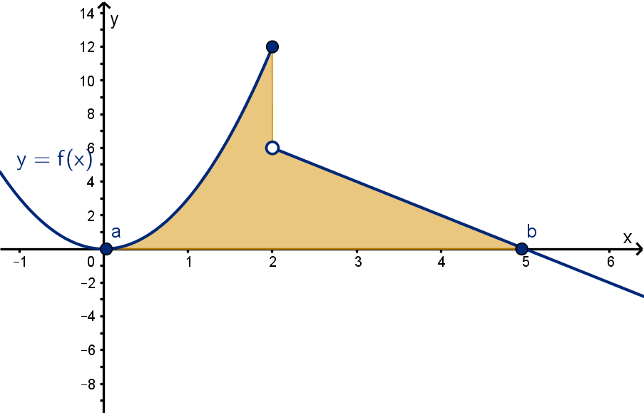
Figure: The area beneath a discontinuous graph
95
Question 2.5.2
How Do We Integrate a Discontinuous Function?
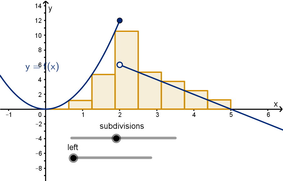
Figure: Rectangle approximations of the area beneath a discontinuous graph
96
Question 2.5.2
How Do We Integrate a Discontinuous Function?
Remarks
We might worry that the approximations are so bad, that the limit
lim
∆x→0
n
X
i=1
f (x
∗
i
)∆x does not exist. Fortunately, it does, as long as
there are only finitely many discontinuities..
f (x) almost has an antiderivative function. F (x) =
Z
x
0
f (t) dt has
derivative f (x) at all x, except perhaps at the points of discontinuity.
97
Question 2.5.2
How Do We Integrate a Discontinuous Function?
We don’t have a form of F (x) that we can evaluate, so how do we
compute
Z
5
0
f (x) dx?
98
Question 2.5.2
How Do We Integrate a Discontinuous Function?
Integrating discontinuous functions
If f (x) is discontinuous at x = c and a ≤ c ≤ b, then
Z
b
a
f (x) dx = lim
t→c
−
Z
t
a
f (x) dx + lim
s→c
+
Z
b
s
f (x) dx
provided that both of these limits exist.
Theorem
If f (x) and g(x) are equal on [a, b] except at a finite number of points,
then
Z
b
a
f (x) dx =
Z
b
a
g(x) dx.
99
Question 2.5.2
How Do We Integrate a Discontinuous Function?
This theorem eliminates the need to use limits in our example
Z
5
0
f (x) dx =
Z
2
0
f (x) dx +
Z
5
2
f (x) dx
=
Z
2
0
3x
2
dx +
Z
5
2
10 −2x dx
Most discontinuities can be handled this way, but there is one type that
will still require limits.
100
Question 2.5.2
How Do We Integrate a Discontinuous Function?
This theorem eliminates the need to use limits in our example
Z
5
0
f (x) dx =
Z
2
0
f (x)
|{z}
=3x
2
dx +
Z
5
2
f (x)
|{z}
= 10 − 2x
except at x = 2
dx
=
Z
2
0
3x
2
dx +
Z
5
2
10 −2x dx
Most discontinuities can be handled this way, but there is one type that
will still require limits.
100
Example 2.5.3
Integrating a Function with a Vertical Asymptote
Definition
When f (x) has a vertical asymptote at c in [a, b] we call
Z
b
a
f (x) dx an
improper integral.
How can we compute
Z
4
0
1
√
x
dx?
101
Example 2.5.3
Integrating a Function with a Vertical Asymptote
Figure: The area beneath a function with a vertical asymptote
Main Idea
To compute an improper integral, we introduce a dummy variable t and
take limit(s) as t → c. If the limit(s) exist, we say the integral
converges. If any do not, we say it diverges.
102
Question 2.5.4
How Can We Compute an Integral over an Unbounded Region?
So far we have been interested in integrals over bounded intervals:
a ≤ x ≤ b. We approximated these with rectangles.
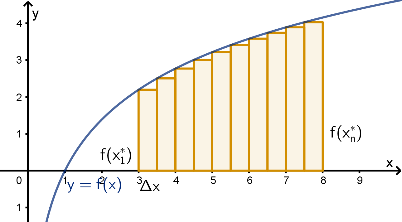
Figure: The area beneath a graph, approximated by rectangles
Consider how this approach would work with an unbounded interval:
a ≤ x.
103
Question 2.5.4
How Can We Compute an Integral over an Unbounded Region?
Rectangles will not approximate the area we want, but we can compute
any finite subsection of it:
Z
t
a
f (x) dx. Like with a discontinuity, we’ll
take a limit.
Definition
An integral of the form
Z
∞
a
f (x) dx is also called an improper integral.
We evaluate it by computing
Z
∞
a
f (x) dx = lim
t→∞
Z
t
a
f (x) dx
assuming this limit exists. If the limit exists we say the improper integral
converges. Otherwise we say it diverges.
Similarly, we can compute
Z
b
−∞
f (x) dx = lim
t→−∞
Z
b
t
f (x) dx.
104
Example 2.5.5
Evaluating an Improper Integral
Compute
Z
∞
2
32
x
3
dx.
105
Example 2.5.5
Evaluating an Improper Integral
Figure: An integral over an unbounded domain
106
Example 2.5.6
An Integral over the Entire Real Line
So far we have looked at intervals unbounded in one direction. If the
interval is (−∞, ∞), the entire real line, then we use the following
definition.
Definition
The improper integral
Z
∞
−∞
f (x) dx is computed:
Z
∞
−∞
f (x) dx =
Z
a
−∞
f (x) dx +
Z
∞
a
f (x) dx
for any number a, so long as both integrals on the right converge. If
either integral diverges, then we say
Z
∞
−∞
f (x) dx diverges as well.
107
Example 2.5.6
An Integral over the Entire Real Line
Let
f (x) =
(
e
x
if x < 1
e
√
x
if x ≥ 1
.
Compute
Z
∞
−∞
f (x) dx.
108
Example 2.5.6
An Integral over the Entire Real Line
Figure: An integral over the real line, broken into two limits
109
Question 2.5.7
Can We Take a Limit of
R
t
−t
f (x ) dx Instead?
The integral
Z
∞
−∞
x
3
dx is a useful test case.
110
Question 2.5.7
Can We Take a Limit of
R
t
−t
f (x) dx Instead?
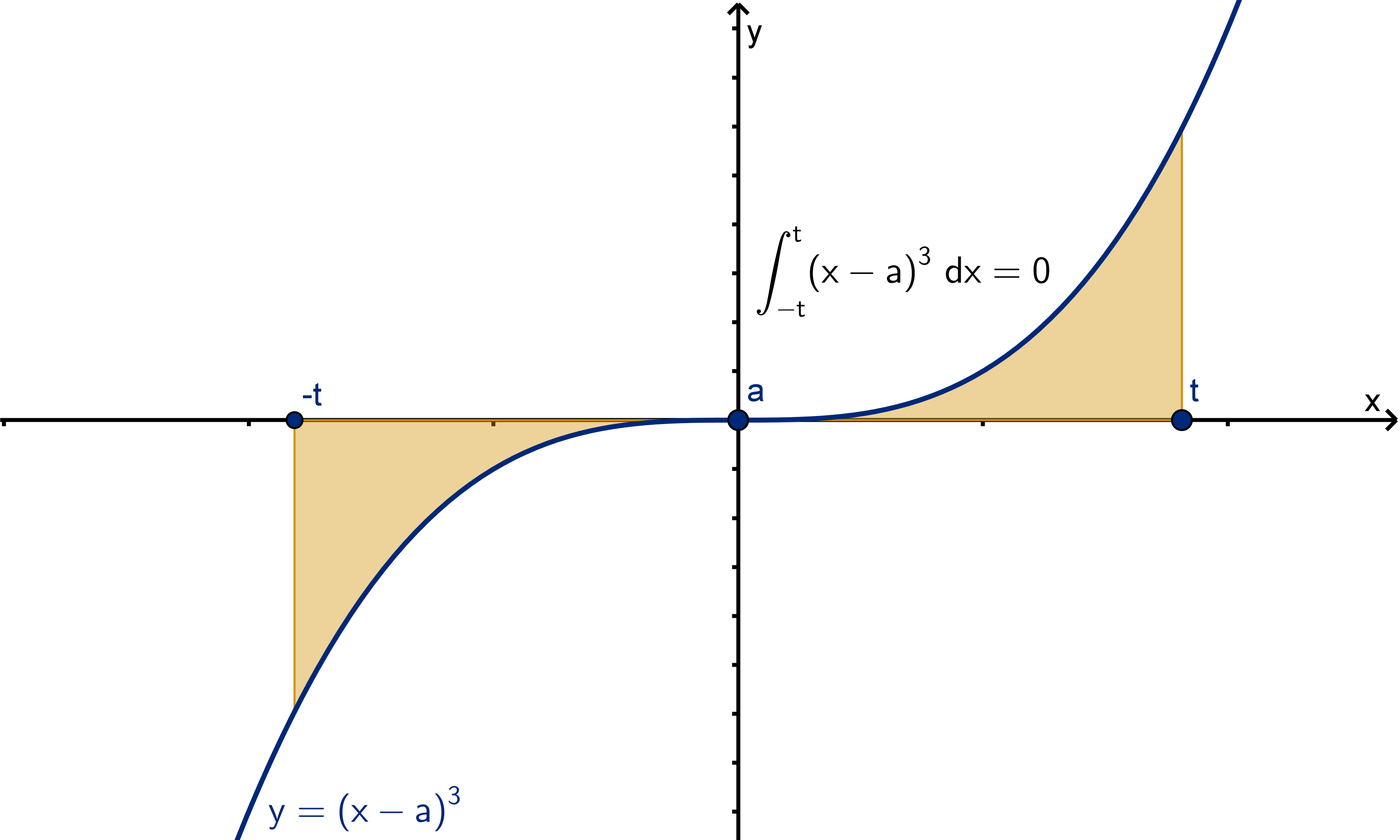
Figure: The area under a functions of the form f (x) = (x − a)
3
111
Question 2.5.7
Can We Take a Limit of
R
t
−t
f (x) dx Instead?
Main Idea
Do not replace the correct definition:
lim
t→−∞
Z
a
t
f (x) dx + lim
t→∞
Z
t
a
f (x) dx
with the “shortcut:”
lim
t→∞
Z
t
−t
f (x) dx
The “shortcut” can suggest that the integral converges, when in fact it
diverges.
112
Synthesis 2.5.8
A Comparison Test
Recall the following theorems
Theorem
If f (x) ≤ g(x) on [a, b] then
Z
b
a
f (x) dx ≤
Z
b
a
g(x) dx.
Theorem
Let a be a real number or ±∞. If F (x) ≤ G (x) for all x near a, then
lim
x→a
F (x) ≤ lim
x→a
G (x).
113
Synthesis 2.5.8
A Comparison Test
Suppose we have a function f (x) whose anti-derivative we don’t know,
and a function g(x) whose anti-derivative we do know. What can the
divergence or convergence of
Z
∞
a
g(x) dx tell us about
Z
∞
a
f (x) dx?
114
Section 2.5
Summary Questions
Q1 What is an improper integral?
Q2 Under what conditions were we able to conclude that
Z
b
a
f (x) dx =
Z
b
a
g(x) dx?
Q3 What does it mean for an improper integral to converge or diverge?
Q4 If we know that
Z
∞
a
g(x) dx converges, what condition on f (x)
would guarantee that
Z
∞
a
f (x) dx converges?
115
Section 2.5
Q26
a How would you write
Z
∞
−∞
1
1 + x
2
dx as a sum of two limits? You
might recall that
Z
1
1 + x
2
dx = tan
−1
x + c. Use this to evaluate
the integral.
b Compare with someone near you. Did you choose the same value of
a when splitting the integral?
c Explain why a different choice of a would not give different values of
the integral. Appeal to a specific integral rule if possible.
116
Section 2.6
Probability
Goals:
1 Test the properties of a probability density function.
2 Use probability density function to describe the underlying random
variable.
3 Use the uniform, exponential, and normal distributions.
4 Compute probabilities and expected values.
Question 2.6.1
What Is a Continuous Probability Distribution?
Why study probability?
The study of inferential statistics is dependent on the ability to compute
probabilities. The basic model for statistical reasoning is:
1 Assume that the type of pattern you’re looking for does not exist (a
null hypothesis).
2 Collect observations.
3 Compute the probability of seeing those observations, given your
assumption.
4 If the probability is very low, then the assumption is probably false.
Probability and inferential statistics are explored thoroughly in later math
courses.
118
Question 2.6.1
What Is a Continuous Probability Distribution?
Definition
A random variable encodes the possible outcomes of a random
selection. We use the notation P(outcome) to denote the probability
that a particular outcome occurs. If an outcome is impossible, we write
P(outcome) = 0. If it is certain we write P(outcome) = 1.
Example
Our outcome can be any expression concerning the random variable, for
instance:
If S is the sum of the rolls of two six-sided dice, then
P(S = 8) =
5
36
.
If T is the number of tails when two coins are flipped then
P(T ≥ 1) =
3
4
.
119
Question 2.6.1
What Is a Continuous Probability Distribution?
We can encode these probabilities with a distribution function. The
value of the function at each number a is the probability that the
outcome is a.
Example
If T is the number of tails obtained from two fair coins then
f
T
(t) =
1
4
if t = 0
1
2
if t = 1
1
4
if t = 2
0 if t = anything else
Notice
The sum of the probabilities adds to 1.
There are only finitely many values of T that are possible.
120
Question 2.6.1
What Is a Continuous Probability Distribution?
What if we wanted to model height with a random variable? No one is
exactly 68 inches tall. Even people who say they are “five feet eight
inches” are slightly taller or shorter. A distribution function like we made
for coins is unsuitable. It would have the property f
H
(h) = 0 for all h.
Definition
A continuous random variable X is a random variable whose outcomes
are real numbers, and whose probability is modeled by a probability
density function f
X
(x) such that
P(a ≤ X ≤ b) =
Z
b
a
f
X
(x) dx.
f
X
(x) must satisfy
1 f
X
(x) ≥ 0 for all x.
2
Z
∞
−∞
f
X
(x) dx = 1
121
Question 2.6.1
What Is a Continuous Probability Distribution?
An integral is the natural way to measure probability.
P(a ≤ X ≤ c) + P(c ≤ X ≤ b) = P(a ≤ X ≤ b)
Z
c
a
f
X
(x) dx +
Z
b
c
f
X
(x) dx =
Z
b
a
f
X
(x) dx
122
Example 2.6.2
Describing a Random Variable from its Density Function
Consider the function
f
X
(x) =
(
1
9
x
2
if 0 ≤ x ≤ 3
0 if x > 3 or x < 0
a Verify that f
X
is a probability density function.
b If f
X
is the density function of X , compute P(X ≥ 2).
c What does f
X
tell us about the likely values of X ?
123
Example 2.6.2
Describing a Random Variable from its Density Function
Figure: The density function of X and the area representing P(X > 2)
124
Example 2.6.2
Describing a Random Variable from its Density Function
Main Ideas
To verify that a function is a probability density function, we need to
check that it is never negative and that it integrates, over the entire
real line, to 1.
We compute the probability that X has an outcome in an interval by
integrating f
X
(x) over that interval.
Outcomes of X where f
X
(x) is large are more likely than outcomes
where f
X
(x) is small.
125
Example 2.6.2
Describing a Random Variable from its Density Function
Figure: The density function of X and the areas that represent the likelihood of
larger and smaller outcomes
126
Question 2.6.3
What Density Functions Arise Naturally?
Definition
Given an interval [a, b], the uniform distribution on [a, b] is given by
f
X
(x) =
(
1
b −a
if a ≤ x ≤ b
0 if x > b or x < a
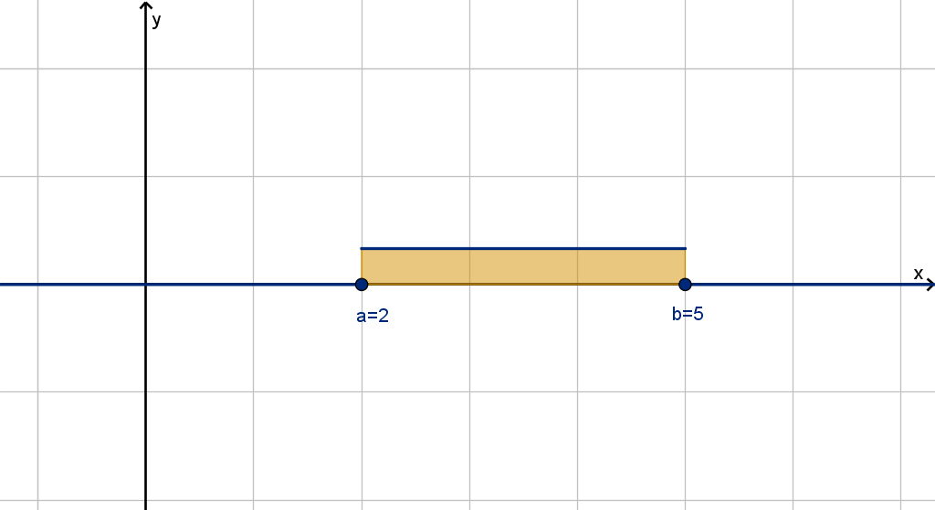
Figure: The density function of a uniform distribution
127
Question 2.6.3
What Density Functions Arise Naturally?
Definition
Suppose an event happens randomly and uniformly at an average rate of
λ times per unit of time (x). Then the amount of time until it next
occurs is given by the exponential distribution:
f
X
(x) =
(
λe
−λx
if 0 ≤ x
0 if x < 0
128
Question 2.6.3
What Density Functions Arise Naturally?
Observe the following
1 Higher λ means that X is likely to be smaller, as the event occurs
sooner.
2 The probability of the event occurring in given interval, given that it
did not occur before that interval, depends only on the length of the
interval.
Figure: The density function of an exponential distribution
129
Question 2.6.3
What Density Functions Arise Naturally?
Definition
The normal distribution is sometimes called a bell curve. Many natural
phenomena are normally distributed. The formula is
f
X
(x) =
1
σ
√
2π
e
−
(x−µ)
2
2σ
2
The anti-derivative of this density function cannot be expressed with
functions that we can evaluate. Instead we can look up values in a table.
The normal distribution has a special role in statistics:
Theorem (The Central Limit Theorem)
The average of any n independent identically distributed random
variables (for instance performing the same experiment n times) will
converge to a normal distribution as n gets large.
130
Question 2.6.3
What Density Functions Arise Naturally?
The parameters in f
X
can be interpreted as follows:
µ is the average value of X . It corresponds to the peak of the bell
curve.
σ is the standard deviation of X . Larger σ means that X has a
larger probability of being far from µ.
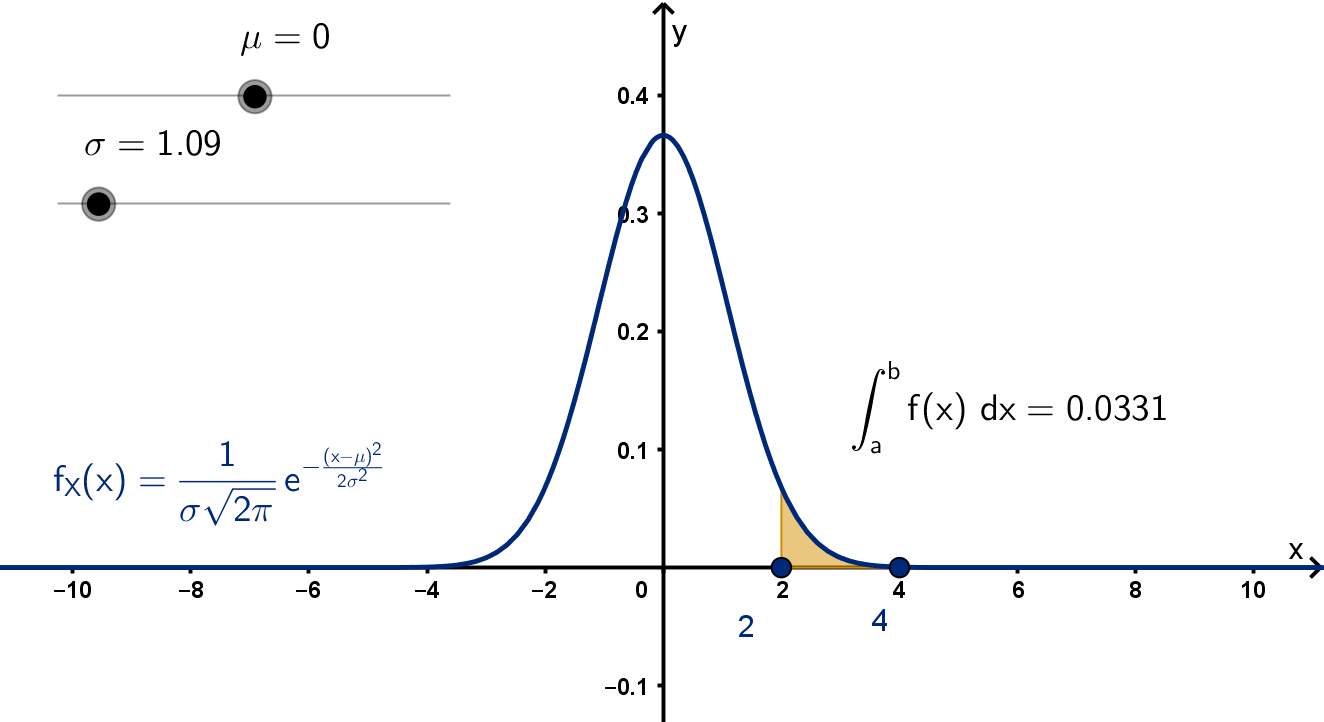
Figure: The density function (bell curve) of a normal distribution
131
Question 2.6.4
What Is the Expected Value of a Random Variable?
The expected value or average value of X describes what the average
result will be, if you let X take a value at random many times. It is
typically denoted E [X ] or with the letter µ.
Example
Suppose we average our rolls of a six-sided die. As the number of rolls n
gets large, we’ll roll each number close to
n
6
times. The sum of the rolls
will be approximately
1
n
6
+ 2
n
6
+ 3
n
6
+ 4
n
6
+ 5
n
6
+ 6
n
6
to compute the average, we divide by n. Fortunately, every term already
has an n.
µ = 1
1
6
+ 2
1
6
+ 3
1
6
+ 4
1
6
+ 5
1
6
+ 6
1
6
= 3.5
132
Question 2.6.4
What Is the Expected Value of a Random Variable?
In general dividing the number of occurrences of the result a in n
evaluations of X will be nf
X
(a). When we divide out n, we obtain the
following weighted average:
Formula
The expected value of a (discrete) random variable X with probability
distribution function f
X
is
E [X ] =
X
x
xf
X
(x)
where x is summed over all possible outcomes of X .
133
Question 2.6.4
What Is the Expected Value of a Random Variable?
To produce the corresponding formula for a continuous random variable,
instead of multiplying each outcome by its probability and summing, we
multiply each output by its density and integrate
Formula
The expected value of a continuous random variable X with probability
density function f
X
is
E [X ] =
Z
∞
−∞
xf
X
(x) dx
134
Example 2.6.5
The Expected Value of a Uniform Random Variable
Compute the expected value of a uniform random variable on [a , b].
135
Example 2.6.5
The Expected Value of a Uniform Random Variable
Main Ideas
E [X ] is typically occurs somewhere in the middle of the possible
outcomes of X . With symmetric density functions, it is the midpoint.
136
Example 2.6.6
The Expected Value of an Exponential Random Variable
a Compute the expected value of a exponential random variable.
b Explain why the role of λ in the answer to a makes sense.
137
Example 2.6.6
The Expected Value of an Exponential Random Variable
Figure: The expected value of a exponential random variable
Main Idea
For asymmetric density functions, E [X ] will not be in the middle of the
range of values. It will be pulled toward regions of higher likelihood.
138
Synthesis 2.6.7
Median Wait Time
Suppose that an exponential random variable models the wait time of a
random caller to a call center.
a What is the median wait time?
b Explain graphically why the median wait time less than the expected
wait time.
139
Synthesis 2.6.7
Median Wait Time
Figure: The median M and expected value µ of an exponential random variable
140
Synthesis 2.6.7
Median Wait Time
Main Idea
The median is the value m such that half the area under y = f
X
(x)
lies on either side of x = m.
We compute the median by setting P(X ≤ m) = 0.5 and solving for
m.
Median is not the same as expected value. y = f
X
(x) may have
more area on one side of E [X ] than the other, if the smaller side’s
area is farther from the middle.
141
Section 2.6
Summary Questions
Q1 Describe the difference between a continuous random variable and a
non-continuous (discrete) one.
Q2 How do we use a probability density function to compute the
probability of an outcome?
Q3 What must be true about a probability density function?
Q4 How do you compute the expected value of a random variable?
142
Section 2.6
Q6
Which of the following probability questions can be answered without
any further information? Explain.
1 If you spin a prize wheel 3 times, what is the probability that my
winnings add up to exactly $80?
2 If you flip two weighted (unfair) coins, what is the probability that
exactly one of them comes up tails?
3 If you pick a random person, what is the probability that her height
is exactly 68 inches?
4 If I spin a wheel of names, what is the probability that it takes
exactly 7 spins to land on my own name?
143
Section 2.7
Functions of Random Variables
Goals:
1 Compute expected values of functions of a random variable.
2 Compute the average value of a function.
3 Compute the variance of a random variable.
Question 2.7.1
What Is a Function of a Random Variable?
Example
Let X be a discrete random variable with probability distribution function
f
X
(x). If Y = g(X ) = X
2
then Y is a random variable and we can
compute its probability distribution function f
Y
(y).
f
X
(x) =
0.1 if x = 0
0.2 if x = 2
0.3 if x = 3
0.4 if x = −2
0 otherwise
f
Y
(y) =
0.1 if y = 0
0.6 if y = 4
0.3 if y = 9
0 otherwise
145
Question 2.7.1
What Is a Function of a Random Variable?
The function g does not need to be algebraically defined.
Example
Let X be a discrete random variable whose outputs are integers from 1 to
100, uniformly distributed (meaning each occurs with probability
1
100
).
Let N give the number of digits of X . Then N has distribution function.
f
N
(n) =
9
100
if n = 1
90
100
if n = 2
1
100
if n = 3
0 otherwise
146
Question 2.7.2
How Do We Compute Expected Value of a Function?
In the case of a discreet random variable, we can compute expected value
directly from the distribution function.
Example
Let X be a discrete random variable whose outputs are integers from 1 to
100, uniformly distributed. Let N give the number of digits of X .
E [N] = (1)
9
100
+ (2)
90
100
+ (3)
1
100
= 1.92
147
Question 2.7.2
How Do We Compute Expected Value of a Function?
Alternately, we could avoid using f
N
by directly applying the digits
function to each outcome X and taking a weighted average.
Example
E [N] = (1)
1
100
+ ···+ (1)
1
100
| {z }
9 times
+ (2)
1
100
+ ···+ (2)
1
100
| {z }
90 times
+ (3)
1
100
= 1.92
148
Question 2.7.2
How Do We Compute Expected Value of a Function?
Formulas
If Y = g [X ] then we can compute E [Y ] from f
X
or from f
Y
.
E [Y ] =
X
outcomes y
i
y
i
f
Y
(y
i
)
E [Y ] =
X
outcomes x
i
g(x
i
)f
X
(x
i
)
Remarks
We can equate these formulas by substituting
f
Y
(y
i
) =
X
g(x
j
)=y
i
f
X
(x
j
).
All that remains is to distribute the y
i
.
Both formulas will get us to the answer, but one of them skips the
step of finding a distribution function for Y .
149
Question 2.7.2
How Do We Compute Expected Value of a Function?
In the case of a continuous random variable X , we might find it difficult
to find the expected value of Y = g (X ) directly. We would need to
Find a density function f
Y
(y) such that
Z
b
a
f
Y
(y) dy = P(a ≤ g (X ) ≤ b)
for all a and b
Integrate E [Y ] =
Z
∞
−∞
yf
Y
(y) dy .
The first step is difficult for any but the simplest functions.
150
Question 2.7.2
How Do We Compute Expected Value of a Function?
Fortunately, there is an integration analogue of substitution and
distributive argument for discrete variables. This allows us to compute
the average outcome of Y as a weighted average of the probabilities of
X .
Theorem
If Y = g (X ) is a function of a continuous random variable X with
density function f
X
(x), then
E [Y ] =
Z
∞
−∞
g(x)f
X
(x) dx
151
Example 2.7.3
Computing the Expected Value of a Function
Consider the random variable X with density function
f
X
(x) =
(
1
9
x
2
if 0 ≤ x ≤ 3
0 if x > 3 or x < 0
What is the expected value of e
X
?
152
Application 2.7.4
The Average Value of a Function
Definition
The average value of a function from x = a to x = b is the expected
value of f (X ), where X is a uniform random variable on [a, b]. The
density function is a constant, so we can factor it out of the integral. We
obtain the formula:
f
ave
=
1
b − a
Z
b
a
f (x) dx.
153
Application 2.7.4
The Average Value of a Function
The signed area under the graph y = f (x) from x = a to x = b is
Area =
Z
b
a
f (x) dx.
The region under the horizontal line y = f
ave
is a rectangle with equal
signed area:
Area = width ×height = (b − a)
1
b − a
Z
b
a
f (x) dx
.
In other words, if we flattened the area under f into a rectangle, f
ave
would be its height.
154
Application 2.7.4
The Average Value of a Function
Figure: The graph of y = f (x) and the constant function y = f
ave
155
Example 2.7.5
Computing The Average Value of a Function
Compute the average value of f (x) = xe
x
2
between x = 1 and x = 3.
156
Application 2.7.6
Variance
Definition
The variance of a random variable X is the expected value of
(X − E [X ])
2
. If X is continuous with density function f
X
(x), we obtain
the formula
Z
∞
−∞
(x − E [X ])
2
f
X
(x) dx
The square root of variance is the standard deviation. Standard
deviation is often denoted by σ, and variance is often denoted by σ
2
.
157
Application 2.7.6
Variance
If the expected value of (x − E [X ])
2
is larger, then X is more likely to be
far from its expected value.
Figure: A density function with less variance and a density function with more
variance
158
Application 2.7.6
Variance
For example, we can compute the variance of X where X is a uniform
random variable on [0, 8].
159
Application 2.7.6
Variance
Remarks
In order to solve for variance, we need to know the expected value.
We may have to compute E [X ] =
Z
∞
−∞
xf
X
(x) dx.
Variance is larger when the area under y = f
X
(x) is spread farther to
both sides, away from E [X ].
160
Section 2.7
Summary Questions
Q1 What kind of object is a function of a random variable?
Q2 How do we compute the expected value of a random variable?
Q3 If someone mentions the “average value” of a function without
mentioning what random variable to use, what do you assume?
Q4 What function’s expected value is the variance?
161
Section 2.7
Q12
Let X be a uniform random variable on [0, 3]. Is Y = X
2
a uniform
random variable on [0, 9]? Provide evidence for your answer.
162
Section 2.7
Q16
Let g(x) = c be a constant function. Let X be a random variable.
Compute E [g(X )].
163