Chapter 6
Multivariable Integration
This chapter introduces integration of functions of more than one variable. It also introduces joint
probability distributions as an application.
Contents
6.1 Double Integrals . . . . . . . . . . . . . . . . . . . . . . . . . . . . . . . . . 410
6.2 Double Integrals over General Regions . . . . . . . . . . . . . . . . . . . . . 424
6.3 Joint Probability Distributions . . . . . . . . . . . . . . . . . . . . . . . . . 437
6.4 Triple Integrals . . . . . . . . . . . . . . . . . . . . . . . . . . . . . . . . . . 463
Section 6.1
Double Integrals
Goals:
1 Approximate the volume under a graph by adding prisms.
2 Calculate the volume under a graph using a double integral.
In single-variable calculus, the definite integral computes a total change from a rate of change.
Moreover, it also solves a geometry problem. This connection means that we can use geometric intuition
to understand integrals better. Integrals of multi-variable functions also allow us to aggregate rates into
totals. To build our intuition, we begin with the geometric problem that they solve.
Question 6.1.1
How Do We Approximate the Volume Under z = f (x, y)?
Begin by remembering our construction of the single-variable definite integral. We approximated
the area under the graph y = f(x) by rectangles. Smaller rectangles give a better approximation, and
we defined the limit of these approximations to be the definite integral.
Z
b
a
f(x)dx = lim
∆x→0
n
X
i=1
f(x
∗
i
)∆x
Figure: The area under y = f(x) approximated by rectangles
Consider a function f(x, y) and a rectangle D = {(x, y) : 0 ≤ x ≤ 4, 0 ≤ y ≤ 2}. We would like
to compute the volume under the part of the graph z = f(x, y) that lies above D. This will need to
be a signed volume, where volume below the xy-plane counts as negative. We approximate this volume
with prisms, because we have a formula for the volume of a prism.
We subdivide D into subrectangles. Over each subrectangle we place a prism. The height of each
prism is the height of the graph above a test point.
410
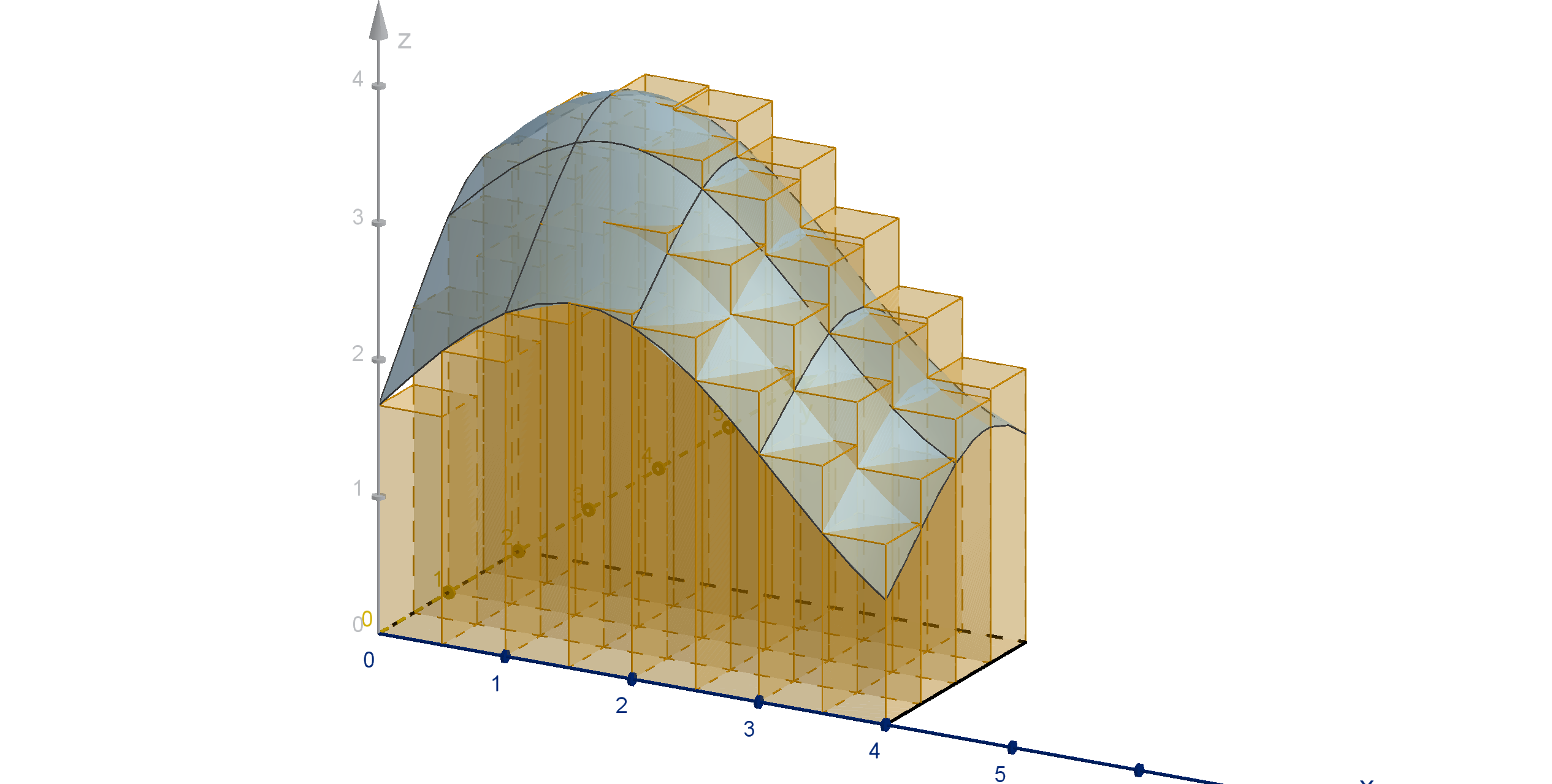
Figure: The volume under z = f (x, y) and the prisms that approximate it
If A is the area of each subrectangle, and (x
∗
i
, y
∗
i
) is the test point in the i
th
subrectangle, then our
approximation is
Volume ≈
n
X
i=1
f(x
∗
i
, y
∗
i
)A.
If our domain is not a rectangle, we may not be able to divide it into subrectangles. Luckily, the
formula for volume of a prism works for any shape base. We can still compute
Volume ≈
n
X
i=1
f(x
∗
i
, y
∗
i
)A
i
.
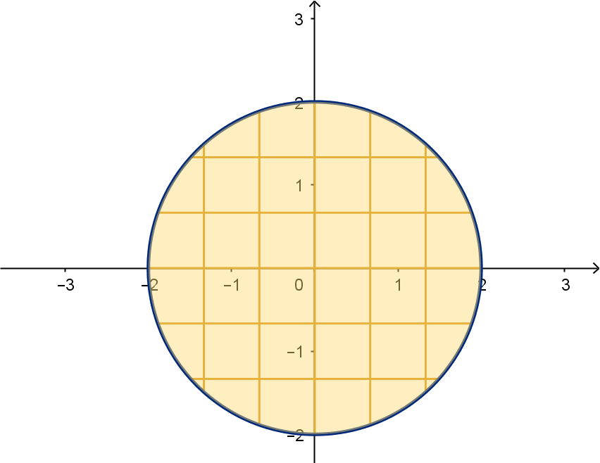
Figure: A domain subdivided into irregular subregions
Notice that instead of a single variable A for the area of all subregions, we need a different area for
each. For each i, A
i
denotes the area of the i
th
subregion.
For a reasonably well-behaved function f(x, y), the actual volume can be computed by taking a limit
of these approximations. We call this limit the double-integral.
411
Question 6.1.1
How Do We Approximate the Volume Under z = f (x, y)?
Definition
Let D be a domain in R
2
. For a given division of D into n subregions denote
A
i
, the area of the i
th
region.
(x
∗
i
, y
∗
i
), any point in the i
th
region
|A| is the diameter of the largest region.
We define the double integral of f(x, y) to be a limit over all possible divisions of D.
ZZ
D
f(x, y)dA = lim
|A|→0
n
X
i=1
f(x
∗
i
, y
∗
i
)A
i
Remark
The diameter of a region is the distance between its two most distant points. Sending the largest
diameter to 0 ensures that all of the regions’ diameters shrink to 0.
Notice that we do not take the limit as the area goes to 0. If only the areas approach 0, the regions
could become long and thin. The test points could all be chosen from one end of the domain which is
unrepresentative of the whole.
Example 6.1.2
Approximating a Double Integral
Consider
ZZ
D
x
2
ydA, where D is the region shown here. Approximate the integral using the division
of D shown, and evaluating f(x, y) at the midpoint of each rectangle.
x
y
1
21
412
Solution
The value of A is the area of each rectangle. In this case that is
A = (1)(0.5) = 0.5.
The test points are the midpoints of each rectangle:
(x
∗
1
, y
∗
1
) = (0.5, 0.25) (x
∗
3
, y
∗
3
) = (1.5, 0.25)
(x
∗
2
, y
∗
2
) = (0.5, 0.75) (x
∗
4
, y
∗
4
) = (1.5, 0.75)
We can expand the sum and evaluate:
Volume ≈
4
X
i=1
f(x
∗
i
, y
∗
i
)A
≈ A
4
X
i=1
f(x
∗
i
, y
∗
i
)
≈ A
f(0.5, 0.25) + f(0.5, 0.75) + f(1.5, 0.25) + f(1.5, 0.75)
≈ 0.5
(0.5)
2
(0.25) + (0.5)
2
(0.75) + (1.5)
2
(0.25) + (1.5)
2
(0.75)
Question 6.1.3
How Do We Evaluate Double Integrals?
We already know another way of computing a volume. We can compute the area of the cross sections
perpendicular to the x-axis. Let the function A(x) denote this area at each x. Then
Volume =
Z
b
a
A(x) dx
A(x) is itself the area under a curve. In a particular cross section, x is constant, and f(x, y) is a function
of y. The area below this graph is the integral
A(x) =
Z
d
c
f(x, y) dy
We can put these together to obtain an iterated integral, an integral whose integrand is itself an
integral.
413
Question 6.1.3
How Do We Evaluate Double Integrals?
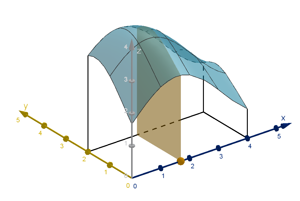
Figure: Cross sections of the region below the graph: z = f (x, y)
This method computes the same signed volume as the double integral we defined. The formal
argument that they are equivalent is called Fubini’s theorem.
Theorem [Fubini’s Theorem]
For any domain D we have
ZZ
D
f(x, y) dA =
Z
b
a
Z
d
c
f(x, y) dy
!
dx
where a and b are the x bounds of D, and c and d are the y bounds of the cross section at each x.
Alternately, we can write
ZZ
D
f(x, y) dA =
Z
d
c
Z
b
a
f(x, y) dx
!
dy
where c and d are the y bounds of D, and a and b are the x bounds of the cross section at each y.
414
Notation
We will generally omit the parentheses and write
Z
b
a
Z
d
c
f(x, y) dydx.
In some cases, rather than figuring out what a, b, c and d are, we will use a hybrid notation. It indicates
a particular order of integration but does not go into details about the bounds of x and y.
ZZ
D
f(x, y)dydx.
Example 6.1.4
Using Fubini’s Theorem
Compute
ZZ
D
x
2
y dA, where D is the region shown here:
x
y
1
21
Solution
The x bounds of this region are 0 ≤ x ≤ 2. The y bounds are 0 ≤ y ≤ 1. We rewrite this as an
integrated integral and solve:
ZZ
D
x
2
y dA =
Z
2
0
Z
1
0
x
2
y dydx (Fubini’s theorem)
=
Z
2
0
x
2
y
2
2
1
y=0
dx (FTC on the inner integral)
=
Z
2
0
x
2
1
2
2
−
x
2
0
2
2
dx (plug in y values)
=
Z
2
0
x
2
2
dx
=
x
3
6
2
x=0
=
8
6
−
0
6
415
Example 6.1.4
Using Fubini’s Theorem
=
4
3
Question 6.1.5
Can We Break a Double Integral into a Product of Single Integrals?
In general, we can’t expect to factor out the inner integral of
RR
D
f(x, y)dydx (using the constant
multiple rule). The y-bounds may depend on x, and the y terms may not factor out of the integrand.
However, for certain functions and domains, this factoring is possible.
Theorem
Z
b
a
Z
d
c
f(x)g(y)dydx =
Z
b
a
f(x)dx
!
Z
d
c
g(y)dy
!
We won’t be able to use this theorem all the time. It has two important requirements:
1 The bounds of integration (a, b, c, d) are constants. We’ll see integrals soon where this is not the
case.
2 The integrand can be factored into a function of x times a function of y. Most two-variable
functions cannot.
Example 6.1.6
Integrating a Product
Use a product decomposition to compute
RR
D
x
2
ydA, where D is the region shown here:
x
y
1
21
416
Solution
ZZ
D
x
2
y dA =
Z
2
0
Z
1
0
x
2
y dydx has constant bounds and the integrand can factor as (x
2
)(y). The
product theorem applies:
Z
2
0
Z
1
0
x
2
y dydx =
Z
2
0
x
2
dx
Z
1
0
ydy
=
x
3
3
2
0
!
y
2
2
1
0
!
=
2
3
3
−
0
3
3
1
2
2
−
0
2
2
=
8
3
1
2
=
4
3
This matches our computation from Example 4.
Remark
The product decomposition does not save us much work in most cases, but it can help us avoid mixing
up the variables.
Application 6.1.7
Rates (per Area)
Single integrals can compute total change given a rate of change.
meters traveled per second −→ total meters traveled.
GDP growth per year −→ total GDP growth.
mass of a chemical produced per second −→ total mass produced.
Double integrals can compute a total from a rate per unit of area. Integrating rainfall per square
kilometer gives the total rain that fell in a watershed.
417
Application 6.1.7
Rates (per Area)
Figure: A rainfall density map
Integrating watts per square meter on a solar array gives the total energy generated.

Figure: Solar panels
By Jud McCranie - Own work, CC BY-SA 4.0
https://commons.wikimedia.org/w/index.php?curid=70132767
Application 6.1.8
Probability
If we generate a data set in which we have measured two variables, then the probability that a
random data point lies in a given region is the double integral of a joint density function over that
area.
418
Figure: A highly correlated set of observations and an uncorrelated joint density function
Section 6.1
Exercises
Summary Questions
Q1
What shape do we use to approximate volume under a surface?
Q2
What formula do we use to compute the exact volume under a graph z = f(x, y)?
Q3
What does Fubini’s Theorem tell us?
Q4
What conditions do you need in order to write a double integral as a product of single integrals?
6.1.1
Q5
Suppose that we are approximating the volume under z = f(x, y) over T , the triangle with
vertices (0, 0), (2, 0) and (0, 1). We’d like to use subregions about 0.25 units long per side. Here
are two options:
Cover as much of T with square prisms as possible, use triangluar prisms in the remaining
spots.
419
Section 6.1
Exercises
Cover as much of T with square prisms as possible, and just forget about the remaining
space.
a
Draw a diagram of where the squares and triangles could reasonably be placed.
b
Suppose the side length of the squares shrinks to be arbitrarilty small. Explain why it does
not matter which of the two options we use in these approximations.
Q6
Let S be the unit square:
S = {(x, y) : 0 ≤ x ≤ 1, 0 ≤ y ≤ 1}
Suppose we approximate
ZZ
S
x dA by n prisms whose bases are rectangles of length 1 in the
x-direction and width
1
n
in the y-direction.
a
How could you pick test points in each rectangle to ensure that the value of this approximation
is 0, no matter what n is?
b
How could you pick test points in each rectangle to ensure that the value of this approximation
is 1, no matter what n is?
c
Does the fact that both of these approximations are possible no matter how many rectangles
we use mean that
ZZ
S
x dA does not exist? Explain.
6.1.2
Q7
Show how to approximate the integral
R
6
0
R
12
3
xy dydx using six 3 unit by 3 unit squares and
using their lower right corners as test points. You do not need to simplify the arithmetic.
Q8
Approximate the value of
R
4
0
R
4
−2
sin
2
(πxy)dydx by dividing the domain into an array of 4 rect-
angles (2 ×2), and evaluating the function at the midpoint of each.
Q9
Consider the integral
Z
6
0
Z
9
5
x
y
dydx.
a
Show how to approximate the integral using six 2 unit by 2 unit squares and using their lower
right corners as test points. You do not need to simplify the arithmetic.
420
b
Explain how you can tell whether your approximation in
a
is an overestimate or underesti-
mate without computing the actual value of the integral.
Q10
Let T be the triangle with vertices (0, 0), (1, 0) and (0, 2). Show how to approximate
ZZ
T
e
x+y
dA
by dividing T into four right triangles with legs of length 1 and
1
2
. Use the midpoint of the
hypotenuses as the test points.
6.1.3
Q11
Let R be the rectangle
R = {(x, y) : 0 ≤ x ≤ 5, 0 ≤ y ≤ 3}.
Let S be the solid region above R and below the graph z = y
2
sin πx + 9. What is the area of
the y = 2 cross-section of S?
Q12
Let R be the rectangle
R = {(x, y) : − 2 ≤ x ≤ 2, −1 ≤ y ≤ 1}.
Let S be the solid region above R and below the graph z = x
2
y + xy
2
. Write a function A(x)
which gives the area of the cross section of S perpendicular to the x-axis at each value of x.
6.1.4
Q13
Let R be the rectangle
R = {(x, y) : 0 ≤ x ≤ 5, 0 ≤ y ≤ 3}.
Compute
ZZ
R
y
2
sin πx + 9 dA
Q14
Let R be the rectangle
R = {(x, y) : − 2 ≤ x ≤ 2, −1 ≤ y ≤ 1}.
Compute
ZZ
R
x
2
y + xy
2
dA.
421
Section 6.1
Exercises
Q15
Evaluate
Z
5
4
Z
3
0
ye
x
dydx.
Q16
Evaluate
Z
10
0
Z
4
2
y
3
− x dydx.
6.1.5
Q17
Let R be the rectangle
R = {(x, y) : − a ≤ x ≤ b, c ≤ y ≤ d}.
Let S be the solid region above R and below the graph z = f(x)g(y). Write a function A(x)
which gives the area of the cross section of S perpendicular to the x-axis at each value of x.
Explain why you can factor the f(x) out of this integral.
Q18
Let R be the rectangle
R = {(x, y) : − 2 ≤ x ≤ 2, −1 ≤ y ≤ 1}.
Explain why the product decomposition theorem does not apply to
ZZ
R
x
2
y + xy
2
dA.
6.1.6
Q19
Let R be the rectangle
R = {(x, y) : 0 ≤ x ≤ 5, 0 ≤ y ≤ 3}.
Write
ZZ
R
y
2
sin πx dA as a product of two single-variable integrals.
Q20
Write
Z
3
−3
Z
5
2
1
y
2
dydx as a product of two single-variable integrals.
422
6.1.7
Q21
A corrugated metal sheet has density of dx, y = 3 + sin 2x kg/m
2
. What is the mass of the
rectangular sheet R = {(x, y) : 0 ≤ x ≤ 4π, 0 ≤ y ≤ 10}?
Q22
The shadow of a tree passes over part of a solar panel each day, covering the bottom of the panel
more of the day than the top. The rate of daily energy generation per unit of area at the point
(x, y) is given by p(x, y) = 8 sin
y +
π
3
kilowatt hours per square meter. Compute the total
power generated per day by the panel whose bounds (in meters) are given by 0 ≤ x ≤ 1 and
0 ≤ y ≤
π
6
.
Synthesis & Extension
Q23
Suppose we wanted to compute the volume above z = f(x, y) and below z = g(x, y) over the
rectangle
R = {(x, y) : a ≤ x ≤ b, c ≤ y ≤ d}.
What double integral would compute this volume?
Q24
Suppose you want to approximate
Z
b
a
Z
d
c
f(x, y)dydx
by rectangles sampled from either upper-left, upper-right, lower-left or lower-right corners. If you
are told that f
x
(x, y) < 0 at all points (x, y), what does that tell you about which approximations
are larger than which?
423
Section 6.2
Double Integrals over General Regions
Goals:
1 Set up double integrals over regions that are not rectangles.
2 Evaluate integrals where the bounds contain variables.
3 Decide when to make
R
dy the outer integral, and compute the change of bounds.
So far, we have computed double integrals over rectangular domains. In this section, we consider
double integrals over more complicated domains.
Example 6.2.1
Integrating Over a Polygon
Let D be the triangle with vertices (0, 0), (4, 0) and (4, 2). Calculate
ZZ
D
4xy dA
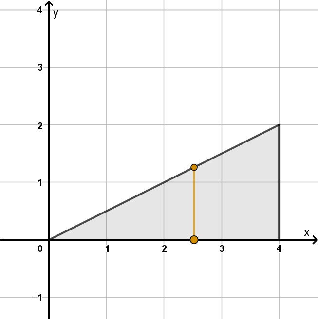
Solution
The naive approach would be to use the x and y bounds of D to write the integral
ZZ
D
4xy dA =
Z
4
0
Z
2
0
4xy dydx
There are a couple reasons to distrust this approach
424
1 These are the same bounds we would use for a rectangle, and D is not a rectangle.
2 The y bounds are supposed to be the bounds of the cross section, and not every cross section
extends from y = 0 to y = 2.
In fact, the y bounds of the cross section depend on which cross section we’re looking at. At x = 1
the cross section has area A(1) =
R
0.5
0
4xy dy. At x = 3 the area is A(3) =
R
1.5
0
4xy dy. Another way
to say this is that the y bounds are a function of x. No matter what x we choose, the lower y bound
appears to be 0. The upper bound always lies on the line from (0, 0) to (4, 2). We can express the
y-values of this line as a function of x by writing its equation: y =
1
2
x. The correct iterated integral is
ZZ
D
4xy dA =
Z
4
0
Z
1
2
x
0
4xy dydx
This may appear harder to solve, but it isn’t. The only difference is that when we apply the fundamental
theorem of calculus to the inner integral, we plug in an expression instead of a number.
ZZ
D
4xy dA =
Z
4
0
Z
1
2
x
0
4xy dydx (Fubini’s theorem)
=
Z
4
0
2xy
2
1
2
x
0
dx (FTC)
=
Z
4
0
2x
1
2
x
2
− 2x(0)
2
dx
=
Z
4
0
x
3
2
dx
=
x
4
8
4
x=0
(FTC again)
=
4
4
8
−
0
4
8
= 32
Main Idea
To find the bounds of a double integral
1 Find the x value where the domain begins and ends. These numbers are the bounds of the outer
integral.
2 Find the functions (of the form y = g(x)) which define the top and bottom of the domain. These
functions are the bounds of the inner integral.
425
Question 6.2.2
What Are the Integral Laws for Double Integrals?
Some single variable integral laws apply to double integrals as well (provided the integrals exist).
1 The sum rule:
ZZ
D
f(x, y) + g(x, y)dA =
ZZ
D
f(x, y)dA +
ZZ
D
g(x, y)dA
2 The constant multiple rule:
ZZ
D
cf(x, y)dA = c
ZZ
D
f(x, y)dA
3 If D is the union of two non-overlapping subdomains D
1
and D
2
then
ZZ
D
f(x, y)dA =
ZZ
D
1
f(x, y)dA +
ZZ
D
2
f(x, y)dA
Example 6.2.3
A Region Without a (Single) Bottom Curve
Let D be the region bounded by y =
√
x, y = 0 and y = x − 6. Calculate
ZZ
D
(x + y) dA.
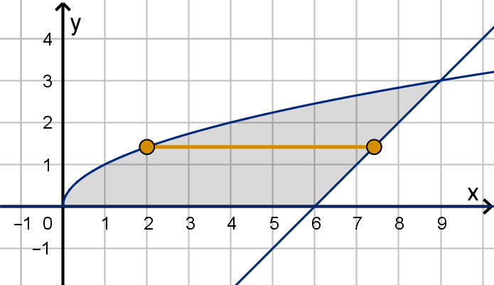
We begin by finding the intersections of these graphs. There are three pairs of graphs to solve for.
√
x = x − 6 0 =
√
x
0 = x − 6
x = (x − 6)
2
0 = x 6 = x
0 = x
2
− 13x − 36
0 = (x − 4)(x − 9)
x = 4 or x = 9
When we square both sides of an equation we have to check our solutions. x = 4 does not satisfy
√
x = x −6 but x = 9 does. Look at the graph of these functions. There is not a single y lower bound
that applies to all cross sections of this region. For some values of x, the lower bound lies on y = 0.
For others it lies on y = x − 6. We will present three solutions to this problem. We’ll only evaluate the
last one.
426
Solution 1
Using the third integral law, we break up D into two subdomains, each of which has a single bottom
curve. The break happens at x = 6 since that is where y = 0 meets y = x − 6.
Z
6
0
Z
√
x
0
(x + y) dA +
Z
9
6
Z
√
x
x−6
(x + y) dydx
Solution 2
D can be written as the region between y = 0 and y =
√
x with a triangle removed. We can use this
to write
ZZ
D
(x + y) dA as a difference of two integrals.
Z
9
0
Z
√
x
0
(x + y) dA −
Z
9
6
Z
x−6
0
(x + y) dydx
Solution 3
Instead of taking cross sections perpendicular to the x-axis we can take cross sections perpendicular
to the y-axis. In this case, we need to know the x bounds of each cross section (as a function of
y). Drawing the horizontal line segments through D at each y, we see that the upper x-bound lies on
y = x −6 and the lower x bound lies on y =
√
x. We need to write these x values as functions of y so
we solve them for y:
y =
√
x y = x − 6
y
2
= x y + 6 = x
The lower y bound for the region is y = 0. The upper y bound is the intersection of y =
√
x and
y = x − 6, where x = 9 and y = 3. Thus we can write
ZZ
D
(x + y) dA =
Z
3
0
Z
y+6
y
2
(x + y) dxdy
=
Z
3
0
x
2
2
+ xy
y+6
y
2
dy
=
Z
3
0
y
2
+ 12y + 36
2
+ y
2
+ 6y −
y
4
2
− y
3
dy
=
Z
3
0
−
1
2
y
4
− y
3
+
3
2
y
2
+ 12y + 18 dy
= −
1
10
y
5
−
1
4
y
4
+
1
2
y
3
+ 6y
2
+ 18y
3
0
427
Example 6.2.3
A Region Without a (Single) Bottom Curve
= −
243
10
−
81
4
+
27
2
+ 54 + 54
=
1341
20
Main Idea
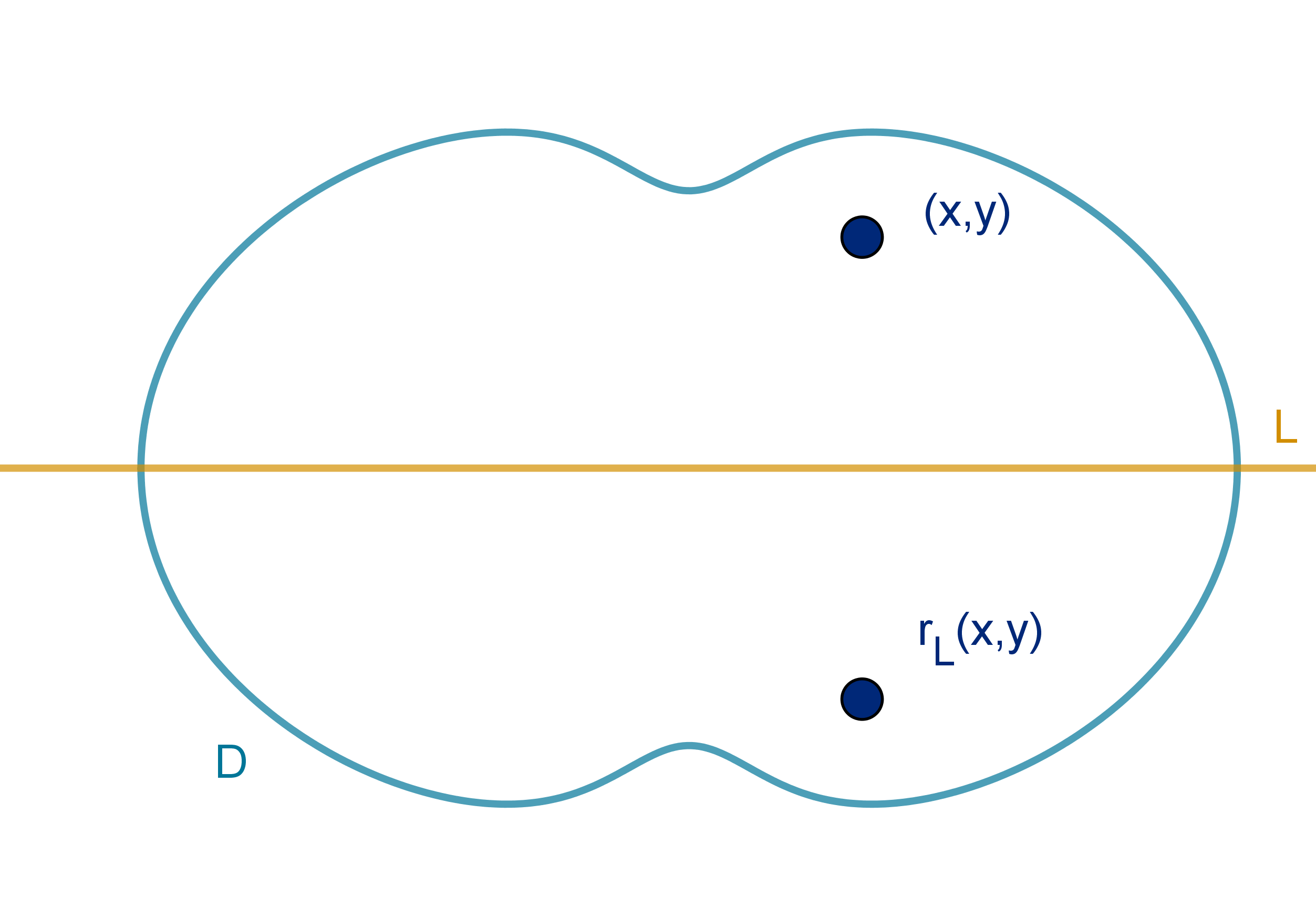
For a region without a single upper or lower curve, the strategies for integrating a function are the same
as the strategies for computing the area.
1 Break the region into two or more pieces, each of which has a single top curve and a single bottom
curve.
2 See if the region has a single left curve (lower x bound) and a single right curve (upper x bound).
If so, solve the bounds for x and change the order of integration.
Example 6.2.4
Using Anti-Symmetry
Let D be the region x
2
+ y
2
≤ 9. Evaluate
ZZ
D
3
√
x
p
y + 3dA.
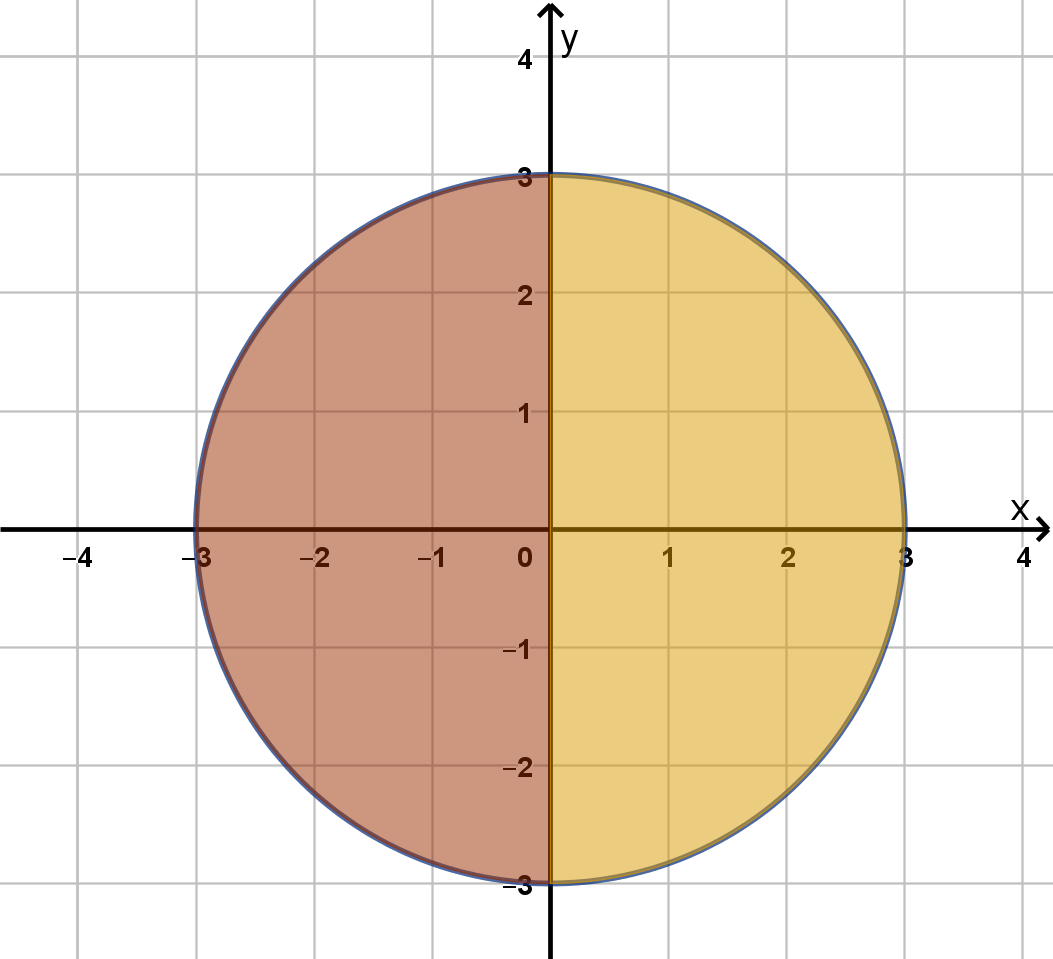
428
Solution
The function f and the domain D both have a particular type of symmetry. D is symmetric about the
y-axis. We can flip the right side of D over onto the left side of D and they match up perfectly. We
can express this transformation in algebra by
(x, y) → (−x, y)
Furthermore, f(x, y) =
3
√
x
√
y + 3 and f(−x, y) =
3
√
−x
√
y + 3 are opposites (they sum to 0). Thus
the height of the graph z = f(x, y) above the left half of D is equal to the depth of the graph below
the right half of D. These two regions have opposite signed volumes. Their sum, which is the integral
over all of D, is 0.
Main Idea
We can argue that an integral
ZZ
D
f(x, y)dA is equal to zero when
1 D is symmetric about some line L. If we folded it over L, one side of D would lie exactly on the
other side.
2 f is antisymmetric about L. For each point (x, y) in D the image of (x, y) across L, denoted
r
L
(x, y) has the property:
f(r
L
(x, y)) = −f(x, y).
429
Example 6.2.5
Using Order to Manipulate the Integrand
Let D be the triangle with vertices (0, 0), (0, 2) and (1, 2).
Calculate
ZZ
D
e
(y
2
)
dA.
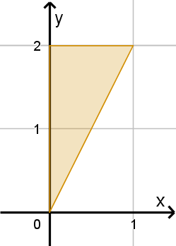
Solution
D is the region above y = 2x and below y = 2 so we can write the integral
ZZ
D
e
(y
2
)
dA =
Z
1
0
Z
2
2x
e
(y
2
)
dydx
The next step is to integrate with respect to y, but e
(y
2
)
does not have an antiderivative that we can
evaluate precisely. The trick in this case is to change the order of integration. The lower x bound is
x = 0 the upper x bound is x =
y
2
.
ZZ
D
e
(y
2
)
dA =
Z
2
0
Z
y
2
0
e
(y
2
)
dxdy
=
Z
2
0
e
(y
2
)
x
y
2
0
dy
=
Z
2
0
e
(y
2
)
y
2
dy
=
Z
4
0
1
4
e
u
du
=
1
4
e
u
4
0
=
e
4
4
−
1
4
u = y
2
y = 0 ⇒ u = 0
du = 2y dy y = 2 ⇒ u = 4
1
4
du =
y
2
dy
u-substitution
Main Idea
If we don’t know the anti-derivative of an integrand with respect to one variable, try switching the order
of integration. Remember to change the bounds too.
430
Application 6.2.6
Area of a Domain
We can use a double integral of f to measure the domain of integration, or compute statistics about
f. Here are two examples.
Theorem
The area of a region D can be calculated:
ZZ
D
1 dA.
This theorem may seem counter-intuitive at first, because a double integral computes a volume, not
an area. However, the volume under a graph of height 1 is equal to 1 times the area of the base. As
long as we change from cubic units to square units, the integral will be numerically equal to the area.
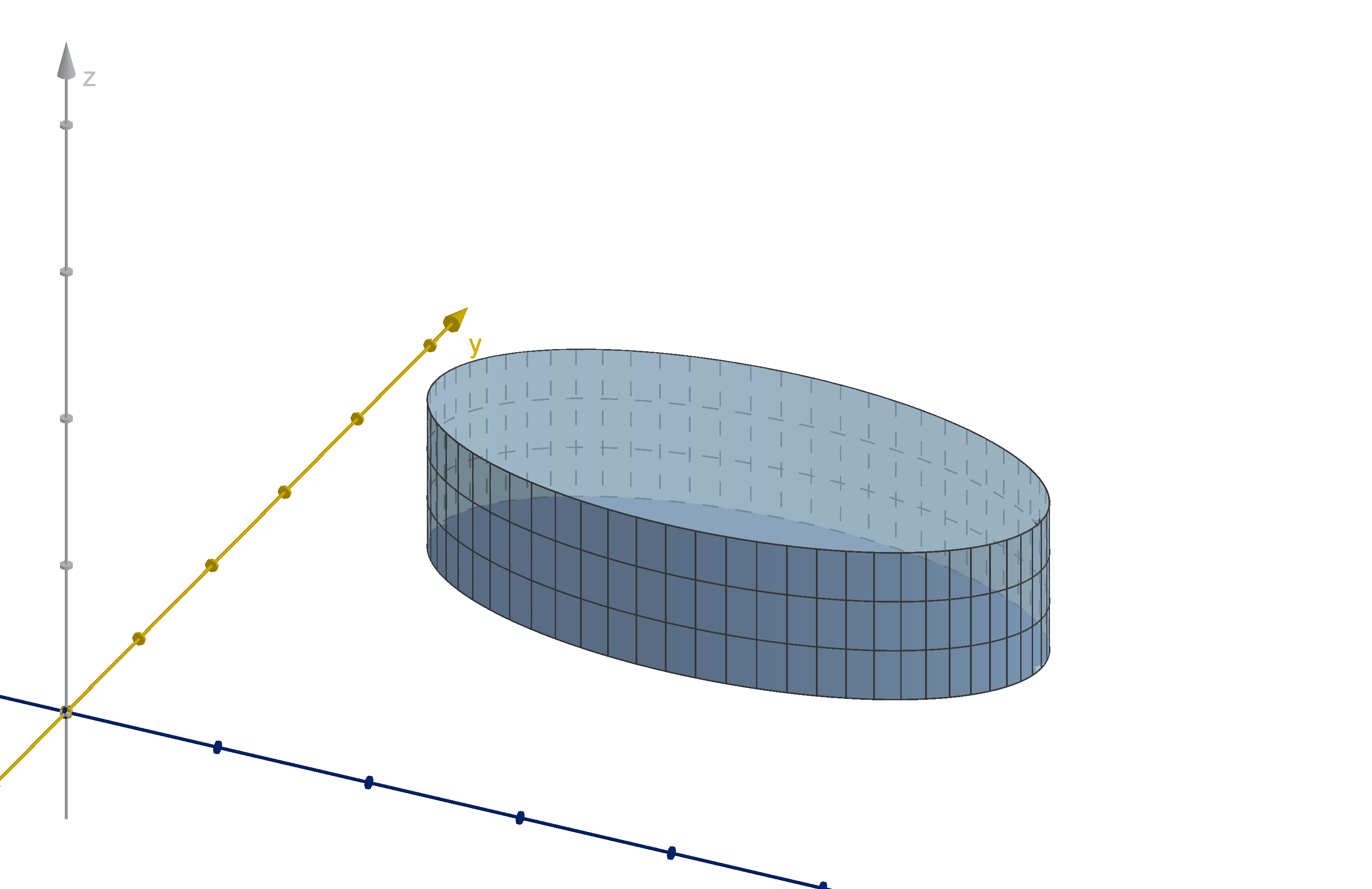
Figure: A solid of height 1 over a domain D
431
Section 6.2
Exercises
Summary Questions
Q1
What are the steps for writing a double integral over a general region?
Q2
How do you decide whether dx or dy is the inner variable?
Q3
What is antisymmetry, and how can we use it to evaluate integrals?
Q4
How can we use a double integral to compute the area of a region?
6.2.1
Q5
If D is the triangle with vertices (0, −2), (4, 0) and (0, 8) calculate
RR
D
x
2
y dA
Q6
Integrate the function f(x, y) = y over the region enclosed by the lines y = 5x, y = 6 − x and
y = x.
Q7
Let f (x, y) be a function and D be the trapezoid with vertices (3, 1), (3, 6), (6, 5) and (6, 4).
Draw D and set up the bounds of
RR
D
f(x, y)dA.
Q8
Let D be the parallelogram with vertices (0, 1), (0, 4), (5, 3) and (5, 6). Let f(x, y) be a contin-
uous function.
a
Set up the bounds of integration of
ZZ
D
f(x, y) dA.
b
Could we save time by computing
Z
5
0
Z
4
1
f(x, y) dydx instead? Explain.
Q9
Let D be the region enclosed by y = 6 − x
2
and y = x. Evaluate
ZZ
D
xe
y
dA.
Q10
If D is the region bounded by y = x
2
and y = 8 − x
2
, set up and calculate
RR
D
x
3
dA.
432
6.2.2
Q11
Let T be the triangle with vertices (0, 3), (7, 10) and (9, 0). Set up the bounds for two intgrals
whose sum is
ZZ
T
f(x, y) dA.
Q12
Let P be the pentagon with vertices (0, 0), (0, 2), (4, 3), (4, 1) and (3, 0).
a
Set up the bounds for two integrals whose sum is
ZZ
P
f(x, y) dA.
b
Set up the bounds for two integrals whose difference is
ZZ
P
f(x, y) dA.
6.2.3
Q13
Let D be the region enclosed by y = ln x, x = 1 and y = 4 − ln x. Set up the integral
ZZ
D
f(x, y) dA
in two different ways, using both orders of dx and dy. Do not evaluate either.
Q14
Let D = {(x, y) : x
2
+ y
2
≤ 9, x ≥ 0}. Draw D and set up
RR
D
f(x, y) dA in two different
ways.
Q15
Consider the region D enclosed by y =
√
x, y = 27
√
x, and y = 90 − x.
a
Rewrite
RR
D
f(x, y) dA as one or more integrals with differential dydx. Do not evaluate.
b
Rewrite
RR
D
f(x, y) dA as one or more integrals with differential dxdy. Do not evaluate.
Q16
Let D = {(x, y) : y ≤ 12 − x
2
, y ≥ x, y ≥ −x}.
a
Rewrite
RR
D
f(x, y) dA as one or more integrals with differential dydx. Do not evaluate.
b
Rewrite
RR
D
f(x, y) dA as one or more integrals with differential dxdy. Do not evaluate.
Q17
Draw the domain of the integral
Z
5
1
Z
10−2x
0
f(x, y) dydx. Then rewrite the integral in the order
dxdy.
433
Section 6.2
Exercises
Q18
Consider the integral
Z
6
−6
Z
0
−
√
36−y
2
x
2
dxdy. Write this integral in the order dydx.
6.2.4
Q19
Let f(x, y) =
3
√
cos x sin y. Argue that
Z
8
−8
Z
√
64−x
2
−
√
64−x
2
f(x, y) dydx = 0.
Q20
Let g(x, y) = x
3
e
y
2
. Argue that
Z
4
−4
Z
3
−3
g(x, y) dydx = 0.
Q21
Let R be the kite with vertices
(1, 1) (5, 7)
(7, 7) (7, 5)
Suppose you wanted to argue that
RR
R
f(x, y)dA = 0 by a symmetry argument. Describe with
a diagram or formula what would need to be true about f(x, y) for such an argument to work.
Q22
Let D be the trapezoid with vertices (0, 5), (6, 5), (2, 0) and (4, 0). Let g(x, y) be some continuous
function.
a
Sketch D and set up the bounds of integration for
RR
D
g(x, y) dA such that you obtain one
integral (not a sum or difference of integrals).
b
If you wanted to use an antisymmetry argument to show that
RR
D
g(x, y) dA = 0 what
would need to be true about g(x, y)? Express your answer as a formula.
Q23
Let h(x) be a one-variable function that takes only positive values. Let f(x, y) be a two-variable
function. Describe the antisymmetry of f that would allow us to conclude that
Z
b
a
Z
h(x)
−h(x)
f(x, y) dydx =
0.
Q24
Suppose you are given that f (x, y) = −f(−y, −x). Over what domains D can we argue by
symmetry that
ZZ
D
f(x, y) dA = 0? Draw an example of one.
434
6.2.5
Q25
Would the method in this example still work, if we instead defined D to have vertices (0, 0),
(1, 0), and (0, 2)? Explain.
Q26
Suggest a domain D over which it would be possible to evaluate
ZZ
D
e
y
3
dA.
Q27
Evaluate
Z
2
0
Z
3
0
ye
xy
dydx.
Q28
Evaluate
Z
3
0
Z
3
x
sin(πy
2
) dydx.
6.2.6
Q29
Use geometry to evaluate
Z
10
0
Z
√
100−x
2
0
dydx.
Q30
Use geomtery to evaluate
Z
8
0
Z
4−
1
2
x
0
dydx.
Synthesis & Extension
Q31
What is the geometric significance of the inner integral in a double integral of the form
Z
b
a
Z
h(y)
g(y)
f(x, y) dxdy?
Q32
Consider the integral
Z
4
−4
Z
6
0
x
3
√
ydydx
a
Show how to approximate the value of this integral, dividing the domain into sub-rectangles
of length 2 units and width 3 units and using the lower right corners as test points. You
should evaluate any functions that appear in your estimate, but you do not need to simplify
the arithmetic.
435
Section 6.2
Exercises
b
Explain in a sentence or two how you can determine the exact value of this integral without
calculating any anti-derivatives.
c
Discuss what test point you could have picked in
a
, such that your approximation would
have computed the exact value of the integral. Note: There are several relevant observations
to make in response to this question.
436
Section 6.3
Joint Probability Distributions
Goals:
1 Integrate a joint density function to calculate a probability.
2 Recognize when random variables are independent.
Some of the most compelling statistical conclusions do not rely on one measurement but on many,
and the relationship between them. Suppose we test a drug by randomly giving different doses to different
participants, then measuring their symptoms. Knowing the likelihood of each level of symptoms doesn’t
tell you whether the drug is effective. Adding in the knowledge of what percentage of test subjects
receive each dosage does not help. Instead you need to know how likely certain pairs of dose and
outcomes are:
(low dose, low symptoms) (low dose, high symptoms)
(medium dose, low symptoms) (no dose, medium symptoms)
If (no dose, high symptoms) and (high dose, low symptoms) are likely enough, then there is a
correlation which points to efficacy of the drug. Individual random variables with individual density
functions cannot model this behavior. We need two-variable density functions and double integrals.
Question 6.3.1
How Do We Use Double Integrals to Compute Probabilities?
Recall how we modeled continuous random variables.
Definition
A function f is a probability density function for a random variable X, if the chance of an outcome
a < X < b is
R
b
a
f(x)dx.
437
Question 6.3.1
How Do We Use Double Integrals to Compute Probabilities?
Definition
A pair (or more) of random variables X and Y , along with the likelihood of various outcomes (X, Y ) is
called a joint distribution. If the space of outcomes is continuous, the distribution is modeled by a joint
probability density function f
X,Y
(x, y) as follows:
P (a ≤ X ≤ b and c ≤ Y ≤ d) =
Z
b
a
Z
d
c
f
X,Y
(x, y) dydx
More generally, for any region D in R
2
P ((X, Y ) lies in D) =
ZZ
D
f
X,Y
(x, y) dA.
Example 6.3.2
Using a Joint Density Function
Suppose the random variables X and Y have the joint density function
f
X,Y
(x, y) =
(
x + y if 0 ≤ x ≤ 1 and 0 ≤ y ≤ 1
0 otherwise
.
Compute the probability that X is at least twice as large as Y .
Solution
We can write “X is at least twice as large as Y ” with the inequality X ≥ 2Y . This is everything below
the line y =
1
2
x Call this region H. We’ll integrate f over this region. This may seem daunting, but
f(x, y) = 0 outside the unit square. We can break H into two subregions, one that lies inside the square
and one that lies outside. A diagram will make it easier to find the bounds.
Figure: The target region H and the unit square of possible outcomes
438
P
Y ≤
1
2
X
=
ZZ
H
x + y dA
=
Z
1
0
Z
1
2
x
0
x + y dydx +
ZZ
the rest of H
0 dA
=
Z
1
0
xy +
y
2
2
1
2
x
0
dx
=
Z
1
0
1
2
x
2
+
1
8
x
2
dx
=
Z
1
0
5
8
x
2
dx
=
5
24
x
3
1
0
=
5
24
Warning
The region of integration in this example has one fourth of the area of the total region of possibilities,
yet the answer was
5
24
not
1
4
. Do not confuse area with probability. Not all outcomes are equally likely
to occur.
Since we got a low probability, relative to area, we can deduce that the probability density in the
region we examined is lower than at some other parts of the domain. That makes sense. The joint
density function x + y is largest in the upper right corner and lowest in the lower left. More of our
triangle was near the lower left than the upper right.
439
Example 6.3.2
Using a Joint Density Function
Exercise
Darmok and Jalad each travel to the island of Tanagra and arrive between noon and 4 PM. Let (X, Y )
represent their respective arrival times in hours after noon. Suppose their joint density function is
f
X,Y
(x, y) =
(
x
32
if 0 ≤ x ≤ 4 and 0 ≤ y ≤ 4
0 otherwise
.
1 What is the value of
R
4
0
R
4
0
f
X,Y
(x, y)dydx?
2 Calculate the probability that Darmok arrives after 2PM.
3 Calculate the probability that Darmok arrives before Jalad.
4 What does the distribution say about when Darmok is likely to arrive? What about Jalad?
5 Write an integral that computes the probability that they arrive within an hour of each other (set
it up, don’t evaluate).
Question 6.3.3
What Is a Marginal Density Function?
Suppose we have a joint density function f
X,Y
(x, y). What if we are only interested in the values
of X? Perhaps we want to compute the expected value. Recall that a density function f
X
(x) of X
satisfies the property
P (a ≤ X ≤ b) =
Z
b
a
f
X
(x) dx
How can we get this function from the joint density function? We can compute P (a ≤ X ≤ b).
P (a ≤ X ≤ b) =
Z
b
a
Z
∞
−∞
f
X,Y
(x, y) dydx
Compare this to the definition of a probability density function. Both compute the same probability.
Both integrate over the same range of x-values. The only way for this to be true for all values of a
and b is if the integrand is the same. This means that the inner integral
Z
∞
−∞
f
X,Y
(x, y) dy is equal to
f
X
(x), the probability density function of X.
440
When we obtain a density function of one random variable from a joint distribution, we call it a
marginal density function.
Theorem
Given a joint distribution X, Y with joint density function f
X,Y
, the individual variables have marginal
density functions:
f
X
(x) =
Z
∞
−∞
f
X,Y
(x, y) dy
f
Y
(y) =
Z
∞
−∞
f
X,Y
(x, y) dx
For each x-value x
0
, the inner integral
Z
∞
−∞
f
X,Y
(x
0
, y) dy is the area of the x = x
0
cross-section
under z = f
X,Y
(x, y). In this figure, we see that larger values of X are more likely, because their
cross-sections have more area.
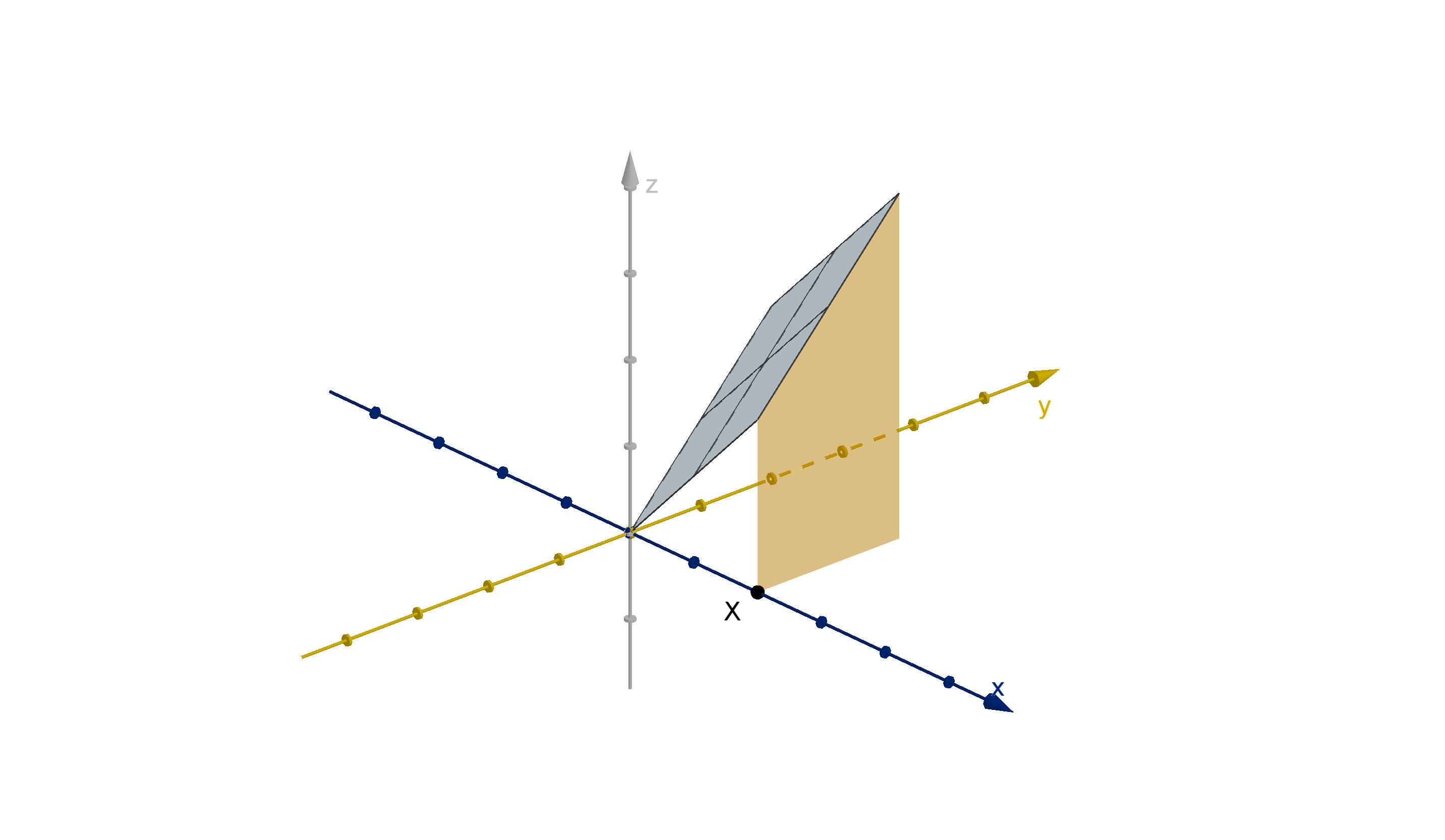
Figure: The marginal density function f
X
(x), represented as cross-sections under z = f
X,Y
(x, y)
Example 6.3.4
Computing Marginal Density Functions
Students at schools around the world compete in a rocketry contest. Rockets are scored based on
the altitude they reach (in meters). Suppose the first and second place altitudes at a randomly chosen
school are modeled by X and Y , which have joint density function
f
X,Y
(x, y) =
(
12−0.012x
1000
y
x
2
−
y
2
x
3
if 0 ≤ x ≤ 1000, 0 ≤ y ≤ x
0 otherwise
441
Example 6.3.4
Computing Marginal Density Functions
a
What can we infer about the possible altitudes of student rockets from this joint density function?
b
Compute the marginal density function of X, the altitude of the first place rocket.
c
What can we conclude about what values of X are more or less likely?
Solution
Figure: The possible outcomes of (X, Y ), and the possible outcomes of Y for each X
a
The maximum altitude of a rocket is 1000m. The second-place rocket always has a lower altitude
than the first-place rocket, which makes sense.
b
For x > 1000 or x < 0, the function f
X,Y
(x, y) = 0 for any choice of Y . For 0 ≤ x ≤ 1000, the
function f
X,Y
(x, y) is piecewise function of y. We can see this in the figure above, f
X,Y
is only
nonzero when 0 ≤ y ≤ x.
f
X
(x) =
Z
∞
−∞
f
X,Y
(x, y) dy
= 0 if x < 0 or x > 1000
=
Z
0
−∞
f
X,Y
(x, y) dy +
Z
x
0
f
X,Y
(x, y) dy +
Z
∞
x
f
X,Y
(x, y) dy if 0 ≤ x ≤ 1000
= 0 +
Z
x
0
12 − 0.012x
1000
y
x
2
−
y
2
x
3
dy + 0
=
12 − 0.012x
1000
Z
x
0
y
x
2
−
y
2
x
3
dy constant multiple rule
=
12 − 0.012x
1000
y
2
2x
2
−
y
3
3x
3
x
0
442
=
12 − 0.012x
1000
x
2
2x
2
−
x
3
3x
3
− 0 + 0
=
12 − 0.012x
1000
1
2
−
1
3
=
2 − 0.002x
1000
f
X
(x) =
(
2−0.002x
1000
if 0 ≤ x ≤ 1000
0 otherwise
c
f
X
(x) has its largest value at x = 0 and shrinks to 0 as x increases to 1000. This indicates that
lower altitudes are much more likely than higher altitudes.
Figure: The marginal density function of X
Figure: The marginal density function of X, represented as an area under the graph of z = f
X,Y
(x, y)
(z-axis not to scale)
Remark
Even though the range of possible outcomes is greater for larger X, the probability of achieving that X
is smaller. We can see this in the cross sections on the joint-density function. Larger values of X have
longer cross sections, but it is the area under the graph z = f
X,Y
(x, y) that matters.
443
Example 6.3.4
Computing Marginal Density Functions
Main Idea
If the range of possible outcomes is limited, then computing f
X
(x) requires us to:
1 make different computations for different ranges of X and
2 within each computation, divide the integral into pieces depending on which values of Y are
possible.
Question 6.3.5
Why Do We Need Joint Distributions?
If we want to communicate about the possible outcomes of X and Y , do we need to give an
expression for f
X,Y
? Maybe the marginal density functions f
X
and f
Y
tell us everything we need to
know about what outcomes are likely. In fact it does not. Marginal density functions cannot tell us how
the likely outcomes of Y change as the outcome of X changes, or vice versa. For instance, perhaps a
patient given a random amount of medicine X is likelier to have smaller symptoms Y when X is larger.
However, in some cases, there is no change at all. No matter what the outcome of X is, the
likelihood of each Y outcome is the same. In this case, the marginal density functions tell us everything
we need to know. This situation is useful to recognize when it occurs, and we have a name for it.
Definition
If the outcomes of Y don’t depend on the outcome of X and vice versa, we say X and Y are indepen-
dent. In this case
P (a ≤ X ≤ b and c ≤ Y ≤ d) =
Z
b
a
f
X
(x) dx
Z
d
c
f
Y
(y) dy
Example
Suppose Darmok and Jalad’s arrival times have the joint density function
f
X,Y
(x, y) =
(
x
32
if 0 ≤ x ≤ 4 and 0 ≤ y ≤ 4
0 otherwise
.
Jalad’s arrival time is uniformly distributed. Darmok’s is triangular. Neither distribution depends on
the arrival time of the other.
444
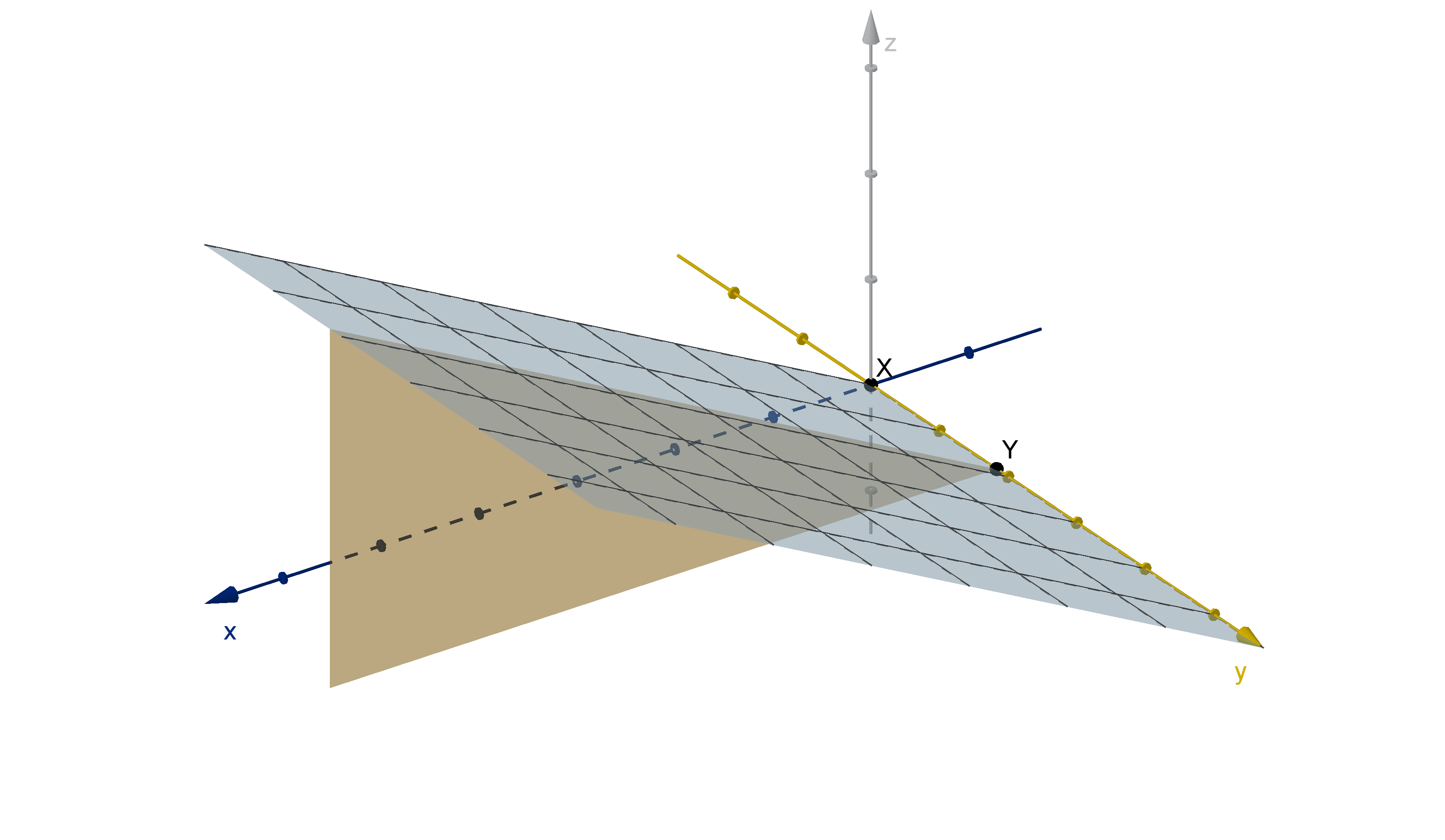
Figure: The density function for Darmok and Jalad’s arrival times
Independence is straightforward to check, and it is closely related to the product decomposition of
a double integral.
Theorem
X and Y are independent, if and only if their joint density function can be written f
X,Y
(x, y) = g(x)h(y),
where
g(x) is a function only of x
h(y) is a function only of y
Remark
g(x) and h(y) can be chosen to be the marginal density functions of X and Y , but they don’t need to
be. As long as a factorization exists, the variables are independent.
Example
Suppose
f
X,Y
(x, y) =
(
3π
12π−8
cos
π
2
x
(2y −y
2
) if 0 ≤ x ≤ 6 and 0 ≤ y ≤ 4
0 otherwise
f
X,Y
(x, y) factors into the marginal density functions
f
X
(x) =
(
π
3π−2
cos
π
2
x
if 0 ≤ x ≤ 6
0 otherwise
f
Y
(y) =
(
3
4
(2y −y
2
) if 0 ≤ y ≤ 4
0 otherwise
Thus we can conclude that X and Y are independent.
445
Question 6.3.5
Why Do We Need Joint Distributions?
We can see independence in the cross sections of z = f
X,Y
(x, y).
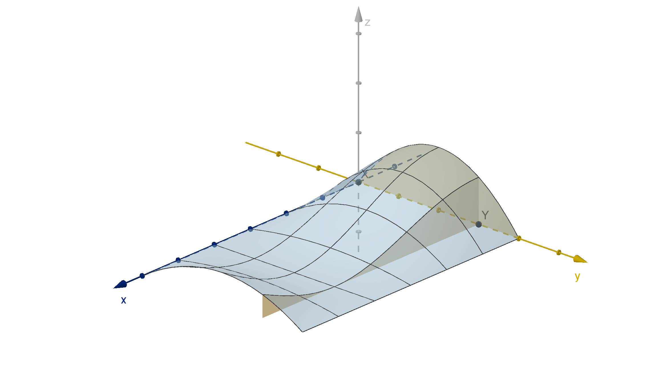
Figure: An independent joint density function and its cross sections
The area of a y = y
0
cross section is f
Y
(y
0
) the likelihood that Y is near y
0
. The shape of the
cross section indicates what X values are likely for that choice of Y . For independent variables, the
X values are distributed the same way no matter what Y value we choose. Mathematically, the cross
section functions are constant multiples of each other. Multiplying by a constant does not change what
portion of the total area lies over a given range of X values.
Question 6.3.6
What Is the Expected Value of a Function of X and Y?
What if we wanted to know the expected value the function g(X, Y ) =
Y
2
X
? By definition, this is
very hard. We would need to write a density function h(t) such that
Z
b
a
h(t) dt = P
a ≤
Y
2
X
≤ b
Notice g(x, y) = a and g(x, y) = b are level curves of g. In this case they solve to
x =
1
a
y
2
x =
1
b
y
2
446
In the case of Darmok and Jalad, the probabilities that h(t) produces would have to integrate to
give the probability that (X, Y ) lies between the level curves:
Figure: The region where a ≤ g(x, y) ≤ b
Even if you did work through the steps to describe the bounds of such a region, you’d need to
1 Write the bounds as a function of a and b, which will be piecewise depending on whether the level
curves exit through the top or the side of the square.
2 Evaluate the integral of f
X,Y
(x, y) over such a region to compute P (a ≤
Y
2
X
≤ b).
3 Use the Fundamental Theorem of Calculus to write an integrand h(t) that integrates to the
probability you found.
4 Integrate
Z
∞
−∞
th(t) dt.
Only then would you know the expected value of g.
Fortunately there is a multivariable analogue to the expected value theorem from single variable
density functions.
Theorem
The expected value of a function g(X, Y ) of two continuous random variables X and Y with joint
density function f
X,Y
(x, y) can be computed:
E[g(X)] =
Z
∞
−∞
Z
∞
−∞
g(x, y)f
X,Y
(x, y) dydx.
447
Example 6.3.7
Expected Value of a Random Variable
A special case of the expected value formula is to compute the expected values of g(x, y) = x or
g(x, y) = y. Suppose X and Y have joint density function
f
X,Y
(x, y) =
(
12−0.012x
1000
y
x
2
−
y
2
x
3
if 0 ≤ x ≤ 1000, 0 ≤ y ≤ x
0 otherwise
Compute E[X].
Solution
E[X] = E[g(X, Y )] where g(x, y) = x. We apply the expected value formula
E[g(X, Y )] =
Z
∞
−∞
Z
∞
−∞
g(x, y)f
X,Y
(x, y) dydx
=
Z
1000
0
Z
x
0
xf
X,Y
(x, y) dydx +
ZZ
everywhere else
xf
X,Y
(x, y) dydx
=
Z
1000
0
Z
x
0
x
12 − 0.012x
1000
y
x
2
−
y
2
x
3
dydx + 0
=
Z
1000
0
x(12 − 0.012x)
1000
Z
x
0
y
x
2
−
y
2
x
3
dydx
=
Z
1000
0
x(12 − 0.012x)
1000
y
2
2x
2
−
y
3
3x
3
x
0
dx
=
Z
1000
0
x(12 − 0.012x)
1000
x
2
2x
2
−
x
3
3x
3
− 0 + 0
dx
=
Z
1000
0
x(12 − 0.012x)
1000
1
2
−
1
3
dx
=
Z
1000
0
x(2 − 0.002x)
1000
dx
=
Z
1000
0
2x − 0.002x
2
1000
dx
=
x
2
1000
−
0.002x
3
3000
1000
0
= 1000 −
2000
3
=
1000
3
448
Main Ideas
We can compute E[X] or E[Y ] by integrating
E[X] =
Z
∞
−∞
Z
∞
−∞
xf
X,Y
(x, y) dydx
E[Y ] =
Z
∞
−∞
Z
∞
−∞
yf
X,Y
(x, y) dydx
If we already have the marginal density function f
X
(x) (or f
Y
(y)), we can use the single-variable
expected value formula:
E[X] =
Z
∞
−∞
xf
X
(x) dx
In fact, we saw this integral partway through our solution. Computing the marginal density function
is nearly equivalent to computing the inner integral in the two-variable expected value formula.
Example 6.3.8
Expected Value of a Function
Compute the expected value of
Y
2
X
where X is Darmok’s arrival time and Y is Jalad’s arrival time.
Assume that X and Y have joint density function:
f
X,Y
=
(
x
32
if 0 ≤ x ≤ 4 and 0 ≤ y ≤ 4
0 otherwise
.
Solution
The expected value is given by
E[Y
2
/X] =
Z
∞
−∞
Z
∞
−∞
y
2
x
f
X,Y
(x, y) dydx
=
Z
4
0
Z
4
0
y
2
x
x
32
dydx because f
X,Y
= 0 outside 0 ≤ x ≤ 4, 0 ≤ y ≤ 4
=
Z
4
0
Z
4
0
y
2
32
dydx
=
Z
4
0
y
3
96
4
0
dx
=
Z
4
0
2
3
dx
449
Example 6.3.8
Expected Value of a Function
=
2
3
x
4
0
=
8
3
Application 6.3.9
Average Value of a Function
Definition
The uniform distribution over a region D in R
2
has the joint density function
f
X,Y
=
(
1
area of D
if (x, y) is inside D
0 if (x, y) is outside D
Like with single variable function, we default to the uniform distribution whenever we average a
function and no specific random variable is specified.
Definition
The average value of a function f over a region D is defined to be the expected value of f(X, Y )
where X, Y are uniformly distributed over D.
f
ave
=
1
Area of D
ZZ
D
f(x, y) dA
Since we can also compute the area of D using a double integral, we can also write
f
ave
=
RR
D
f(x, y) dA
RR
D
1 dA
450
Application 6.3.10
Covariance and Correlation
One of the most useful things to know about a pair of random variables is whether they are correlated,
whether high values of one tend to correspond to high values (or low values) of the other. We can measure
this by examining the expected value of a specific function, which is positive when X and Y are both
above average or both below average, and negative for pairs when one is above and the other is below.
Definition
The expected value of (X −E[X])(Y −E[Y ]) is called the covariance of X and Y , denoted cov(X, Y ).
1 If cov(X, Y ) > 0, higher values of X tend to be correlated with higher values of Y .
2 If cov(X, Y ) < 0, higher values of X tend to be correlated with lower values of Y .
3 If cov(X, Y ) = 0, X and Y are uncorrelated.
To test this, we can look at a type of joint distribution whose correlation we already understand.
Suppose X and Y are independent. Then outcomes of X should not depend on outcomes of Y . The
joint density function can be written f(x, y) = g(x)h(y). We can use our integral rules to see that
covariance is always 0, matching our intuition.
cov(X, Y ) =
Z
∞
−∞
Z
∞
−∞
(x − E[X])(y − E[Y ])f
X,Y
(x, y) dydx
=
Z
∞
−∞
Z
∞
−∞
(x − E[X])(y − E[Y ])g(x)h(y) dydx
=
Z
∞
−∞
(x − E[X])g(x) dx
Z
∞
−∞
(y −E[Y ])h(y) dy
=
Z
∞
−∞
xg(x) dx − E[X]
Z
∞
−∞
yh(y) dy − E[Y ]
= (0)(0)
Covariance on its own does not allow us to compare whether one joint distribution is better correlated
than another. A joint distribution could have a large covariance because the variables are consistently
correlated, or because X (or Y ) has high variance (meaning X is generally farther from E[X]). To
control for the latter effect we often compute:
Pearson’s Correlation
ρ
X,Y
=
cov(X, Y )
σ
X
σ
Y
Where the σs are standard deviations.
ρ returns a value between −1 and 1 which is one measure of how well-correlated two random variables
are.
451
Section 6.3
Exercises
Summary Questions
Q1
How do we use a joint density function to compute the probability of a certain set of outcomes?
Q2
What is a marginal density function and how do we compute it?
Q3
What does it mean for two random variables to be independent?
Q4
How can we tell from the graph of a joint density function that the two random variables are
independent?
6.3.1
Q5
Given a joint density function f
X,Y
(x, y), what does
Z
1
0
Z
x
0
f
X,Y
(x, y) dydx
compute?
Q6
Suppose X and Y have the joint density function
f
X,Y
(x, y) =
(
ax if 0 ≤ x ≤ 4 and 0 ≤ y ≤ 5
0 otherwise
What is the value of the number a?
452
6.3.2
Q7
Suppose X and Y have the joint density function
f
X,Y
(x, y) =
(
y
2
18
if 0 ≤ x ≤ 2 and 0 ≤ y ≤ 3
0 otherwise
Compute the probability that X + Y is greater than 3.
Q8
Suppose X and Y have the joint density function
f
X,Y
(x, y) =
(
x + y if 0 ≤ x ≤ 1 and 0 ≤ y ≤ 1
0 otherwise
Compute the probability that X and Y differ by at least
1
2
.
Q9
Suppose X and Y have the joint density function
f
X,Y
(x, y) =
(
4−x+y
32π
if x
2
+ y
2
≤ 8
0 otherwise
a
What values of (X, Y ) are possible?
b
Among the possible values of (X, Y ), describe which are more or less likely than others.
c
Set up an integral or integrals that would compute the probability that Y > X. You don’t
need to evaluate it.
Q10
Suppose we perform an experiment in which a pair of strangers find an amount of money on
the ground. Suppose X and Y are continuous random variables that model the portion of the
money (0 =none, while 1 = all) that each person keeps. Any money not kept is turned into the
authorities. Suppose the joint density function of X and Y is
f
X,Y
(x, y) =
(
24xy if x ≥ 0, y ≥ 0, and x + y ≤ 1
0 otherwise
a
In a few sentences, interpret what this density function says about which outcomes are likely
and which are not. Feel free to include any comments on human nature that you need to
get off your chest.
b
Set up an integral (or integrals) that computes the probability that each person takes at
most twice as much as the other. Do not evaluate.
453
Section 6.3
Exercises
6.3.3
Q11
Let T be the triangle with vertices (1, 2), (4, 0) and (3, 5). If X and Y are a joint distribution
with a density function f
X,Y
that is nonzero on T and zero everywhere else. For what values of
x is the marginal density function f
X
(x) nonzero? Illustrate with a diagram.
Q12
Let D be the region between y = x
2
and y = 2x + 15. If X and Y are a joint distribution with
a density function f
X,Y
that is nonzero on D and zero everywhere else. For what values of y is
the marginal density function f
Y
(y) nonzero? Illustrate with a diagram.
Q13
Suppose that X and Y are a joint distribution whose density function f
X,Y
is nonzero in the disk
x
2
+ y
2
≤ 1 and nowhere else. If the marginal density function of X is the density function of a
uniform random variable, what does this tell you about where the function f
X,Y
(x, y) is higher
and lower?
Q14
Suppose X and Y have joint density function
f
X,Y
=
(
g(y) if a ≤ x ≤ b and c ≤ y ≤ d
0 otherwise
where g is a function only of y. What is the marginal density funtion of X? Justify your answer,
preferably without actually evaluating any integrals.
6.3.4
Q15
Suppose the random variables X and Y have the joint density function
f
X,Y
(x, y) =
(
x + y if 0 ≤ x ≤ 1 and 0 ≤ y ≤ 1
0 otherwise
.
Compute the marginal density function of X.
Q16
Suppse X and Y have joint density function
f
X,Y
(x, y) =
(
4xy −2x − 2y + 2 if 0 ≤ x ≤ 1, 0 ≤ y ≤ 1
0 otherwise
a
Compute the marginal density function f
X
(x).
454
b
Compute the marginal density function f
y
(y).
c
What familiar kind of random variables are X and Y ?
Q17
Let T be the triangle with vertices (0, 0), (1, 0) and (0, 1). Let X and Y have joint density
function
f
X,Y
(x, y) =
(
6x if (x, y) is in T
0 otherwise
Compute the marginal density function of X.
Q18
Suppose X and Y have joint density function
f
X,Y
(x, y) =
(
15y if x
2
≤ y ≤ x
0 otherwise
a
Draw the region of possible outcomes of (X, Y ) in R
2
.
b
Compute the marginal density function of X.
6.3.5
Q19
Suppose X and Y are independent. Their joint density function f
X,Y
(x, y) has the values
f
X,Y
(3, 7) = 0.1 f
X,Y
(5, 7) = 0.15f
X,Y
(5, 2) = 0.21
What is f
X,Y
(3, 2)?
Q20
How does the distribution of Y change as X takes different values, given the following joint
density function?
f
X,Y
(x, y) =
(
x + y if 0 ≤ x ≤ 1 and 0 ≤ y ≤ 1
0 otherwise
455
Section 6.3
Exercises
Are X and Y independent?
Q21
Suppose X and Y are independent random variables. If their joint density function f
X,Y
(x, y) is
0 except on D, what can we say about the shape of D?
Q22
f
X,Y
(x, y) is a joint density function for a pair of independent variables X and Y . Here is a
picture of the x = 2 cross section of z = f
X,Y
(x, y).
a
Describe what values of Y are more or less likely when X = 2.
b
Assume f
X,Y
(x, y) is not always 0 at x = 5. Describe what values of Y are more or less
likely when X = 5.
c
How is the shape of the x = 2 cross section of z = f
X,Y
(x, y) related to the x = 5 cross
section of z = f
X,Y
(x, y)?
456
6.3.6
Q23
Let X and Y be random variables with joint density function f
X,Y
(x, y) and let D be the
distance from (X, Y ) to the origin. What region would we need to integrate over to compute
P (1 ≤ D ≤ 2)?
Q24
Let X and Y be random variables with joint density function f
X,Y
(x, y) and let Z be the difference
X − Y . What region would we need to integrate over to compute P (0 ≤ Z ≤ 5)?
Q25
Use the expected value formula to show that if Z
1
and Z
2
are both functions of X and Y , then
E[Z
1
+ Z
2
] = E[Z
1
] + E[Z
2
].
Q26
Let T be the triangle with vertices (0, 0), (4, 0) and (0, 4). Suppose X and Y are random variables
with joint density function
f
X,Y
(x, y) =
(
1
8
if (x, y) is in T
0 otherwise
Let Z = X + Y .
a
Write a function G(z) which gives the probability that Z < z.
b
Compute g(z) =
dG
dz
. Explain why P (a ≤ Z ≤ b) =
R
b
a
g(z) dz.
c
Use g to directly compute the expected value of Z.
d
Compute the expected value of Z instead using our multivariable expected value of a function
formula.
6.3.7
Q27
Suppose X and Y have joint density function
f
X,Y
(x, y) =
(
12−0.012x
1000
y
x
2
−
y
2
x
3
if 0 ≤ x ≤ 1000, 0 ≤ y ≤ x
0 otherwise
Compute E[Y ]
457
Section 6.3
Exercises
Q28
Suppose the random variables X and Y have the joint density function
f
X,Y
(x, y) =
(
x + y if 0 ≤ x ≤ 1 and 0 ≤ y ≤ 1
0 otherwise
.
Compute E[Y ].
Q29
Darmok and Jalad’s arrival times X and Y have the joint density function
f
X,Y
(x, y) =
(
x
32
if 0 ≤ x ≤ 4 and 0 ≤ y ≤ 4
0 otherwise
.
What is the expected arrival time of Darmok?
Q30
Suppose the joint density function of X and Y is
f
X,Y
(x, y) =
(
24xy if x ≥ 0, y ≥ 0, and x + y ≤ 1
0 otherwise
. What is the expected value of X?
6.3.8
Q31
Suppose the random variables X and Y have the joint density function
f
X,Y
(x, y) =
(
x + y if 0 ≤ x ≤ 1 and 0 ≤ y ≤ 1
0 otherwise
.
Compute the expected value of XY .
Q32
Darmok and Jalad’s arrival times X and Y have the joint density function
f
X,Y
(x, y) =
(
x
32
if 0 ≤ x ≤ 4 and 0 ≤ y ≤ 4
0 otherwise
.
Darmok is trying to break his habit of arriving late. He has agreed to donate 120 credits to a
local charity for each hour Jalad has to wait for him (prorated across partial hours). Assuming
that this incentive has no effect on their arrival times, what is the expected donation?
458
Q33
Suppse X and Y have joint density function
f
X,Y
(x, y) =
(
4xy −2x − 2y + 2 if 0 ≤ x ≤ 1, 0 ≤ y ≤ 1
0 otherwise
Compute the expected value of X
2
Y
2
.
Q34
The longitude and latitude of a meteorite landing are random variables X degrees and Y degrees
with joint density function
f
X,Y
(x, y) =
(
8100−y
2
349920000
if − 180 ≤ x ≤ 180 and − 90 ≤ y ≤ 90
0 otherwise
a
Write an integral that computes the probability that a meteorite lands within 20 degrees
longitude of the prime meridian (x = 0). Do not evaluate it.
b
What does this density function say about where a meteorite is likely or unlikely to strike?
Answer in a few sentences.
c
Suppose a perverse lottery is established that pays out 30 dollars minus the distance in
degrees from the south pole (y = −90), if the meteorite strikes within 30 degrees of the
south pole. Otherwise it pays out nothing. Set up an integral that computes the average
payout from this lottery. Do not evaluate.
6.3.9
Q35
Compute the average value of the function f(x, y) = 2y on the unit disc x
2
+ y
2
≤ 1.
Q36
Compute the average value of the function f(x, y) = y on the region enclosed by y = x
2
and
y = 16.
Q37
Compute the average value of the function f(x, y) = xy on the triangle with vertices (0, 0), (4, 0)
and (0, 8).
Q38
Compute the average value of the function f(x, y) = x
2
on the triangle with vertices (−2, 0),
(2, 0) and (0, 2).
459
Section 6.3
Exercises
6.3.10
Q39
Recall our friends Darmok and Jalad arriving in Tanagra between noon and 4 PM. The joint
density function of their respective arrival times (X, Y ) is
f
X,Y
=
(
x
32
if 0 ≤ x ≤ 4 and 0 ≤ y ≤ 4
0 otherwise
.
We found that E[X] =
8
3
and E[Y ] = 2. Consider the function g(X, Y ) =
X −
8
3
(Y − 2).
a
Draw the domain of possible values of (X, Y ) At what points in this domain is g positive?
Where is it negative?
b
Could you argue, using the laws of integrals instead of a computation, that E[g(X)] = 0?
Q40
Suppose X and Y have joint density function
f
X,Y
(x, y) =
(
x + y if 0 ≤ x ≤ 1 and 0 ≤ y ≤ 1
0 otherwise
a
Compute E[X] and E[Y ].
b
Compute the covariance of X and Y .
c
What does your answer to
b
suggest about how X and Y are correlated?
Synthesis & Extension
Q41
Suppose D is the region enclosed by 6x−x
2
and the x-axis. Let X and Y are the uniform desntiy
function over D. Let f
X
(x) be the marginal density function of X.
a
What values of X are possible outcomes? What values are impossible?
b
What values of X and more likely and what values are less likely? Justify your answer.
Q42
If X and Y have a uniform joint distribution over some region D, can X and Y be correlated?
Explain or demonstrate.
460
Q43
Suppose on a trip to the movies, the number of minutes you wait in line for tickets (X) and
the number of minutes you wait in line for snacks (Y ) are random variables with joint density
function:
f
X,Y
(x, y) =
(
12x−x
2
+10y−y
2
4880
if 0 ≤ x ≤ 12 and 0 ≤ y ≤ 10
0 otherwise
a
Are X and Y independent? Justify your answer in a sentence or two.
b
Compute the probability that the ticket line takes less than 5 minutes. You don’t need to
simplify the arithmetic.
c
You decide to pay a friend 25 cents per minute to wait in line for snacks while you wait for
the tickets. If you’re still in line when she gets the snacks, she brings them to you and you
pay her. If she’s still in line when you get tickets, you pay her and take her place. Write an
integral or integrals that compute the expected (average) amount you will pay her. Do not
evaluate.
Q44
When you go to the movies, you have to wait in line for tickets, and then to buy snacks. You
model the ticket wait (in minutes) with the random variable X. You model the snack wait with
the random variable Y . Suppose X and Y have the joint density function
f
X,Y
(x, y) =
(
50e
−5x−10y
if 0 ≤ x and 0 ≤ y
0 otherwise
.
a
Compute the probability that you wait a total of no more than 15 minutes in both lines.
b
Are the X and Y in this problem indepedent?
c
Is the independence of X and Y a reasonable assumpton? Explain.
Q45
Darmok and Jalad have agreed to meet up again at Tanagra. Darmok’s arrival time (in hours)
after noon is denoted by the random variable X, while Jalad’s is denoted by the random variable
Y . X and Y have the joint density function
f
X,Y
(x, y) =
(
y
6x
2
if 1 ≤ x ≤ 4 and 0 ≤ y ≤ 4
0 otherwise
a
Describe the possible arrival times of Darmok and the possible arrival times of Jalad.
b
Compute the probability that Darmok arrives at least two hours after Jalad.
461
Section 6.3
Exercises
c
Darmok and Jalad leave Tanagra at exactly 6PM. Write an integral or integrals that compute
the average amount of time they spend together at Tanagra. Do not evaluate your integral(s),
but your integrand(s) should be functions whose antiderivative(s) are well known.
Q46
Let
D = {(x, y) : x
2
+ y
2
≤ 4, y ≥ 0}
Suppose X and Y have joint density function
f
X,Y
(x, y) =
(
3y
16
if (x, y) is in D
0 otherwise
a
Compute the marginal density function of Y
b
What integral would compute the expected value of X? How do you know the value of this
integral without computing it?
Q47
Suppose we wish to approximate
R
6
0
x
2
dx by dividing the domain into two equal subintervals.
Suppose the test points for each subinterval are independently chosen, uniformly distributed ran-
dom variables on their respective subintervals. Produce an integral that computes the probability
that this approximation overestimates the actual value of the integral.
Q48
Suppose X and Y are independent, and their joint density function is written as a product
f
X,Y
(x, y) = g(x)h(y). How is the marginal density function f
X
(x) related to g(x)?
462
Section 6.4
Triple Integrals
Goals:
1 Set up triple integrals over three-dimensional domains.
2 Evaluate triple integrals.
The theory of integrating a two-variable function extends without much trouble to functions of more
variables. Visualizing the domains and writing bounds of integration is a much greater challenge. Any
function whose domain is a piece of the real world needs (at least) three variables. Joint density functions
can also relate any number of random variables. In both cases, a triple integral allows us to aggregate
a rate (per unit of volume) to compute a total over the domain in question.
Question 6.4.1
How Do We Integrate a Three-Variable Function?
A triple integral is a natural extension of the double integral. A good exercise is to compare the two
definitions, point by point.
Definition
Given a domain D in three dimension space, and a function f (x, y, z). We can subdivide D into regions
V
i
is the volume of the i
th
region.
(x
∗
i
, y
∗
i
, z
∗
i
) is a point in the i
th
region.
V is the diameter of the largest region.
We define the triple integral of f over D to be the following limit over all possible divisions of D:
ZZZ
D
f(x, y, z) dV = lim
V →0
n
X
i=1
f(x
∗
i
, y
∗
i
, z
∗
i
)V
i
Fubini’s theorem applies to triple integrals as well. We write them as iterated integrals.
Theorem
ZZZ
D
f(x, y, z)dV =
Z
x
2
x
1
Z
y
2
y
1
Z
z
2
z
1
f(x, y, z) dzdydx
where
z
1
and z
2
are the bounds of z, which may be functions of x and y.
y
1
and y
2
are the bounds of y, which may be functions of x.
x
1
and x
2
are the bounds of x. They are numbers.
The variables of can also be reordered, with the bounds defined analogously.
463
Question 6.4.1
How Do We Integrate a Three-Variable Function?
Example 6.4.2
Integrating Over a Prism
Let R = {(x, y, z) : 0 ≤ x ≤ 4, 0 ≤ y ≤ 2, 0 ≤ z ≤ 3}. Compute
ZZZ
R
3zy + x
2
dV .
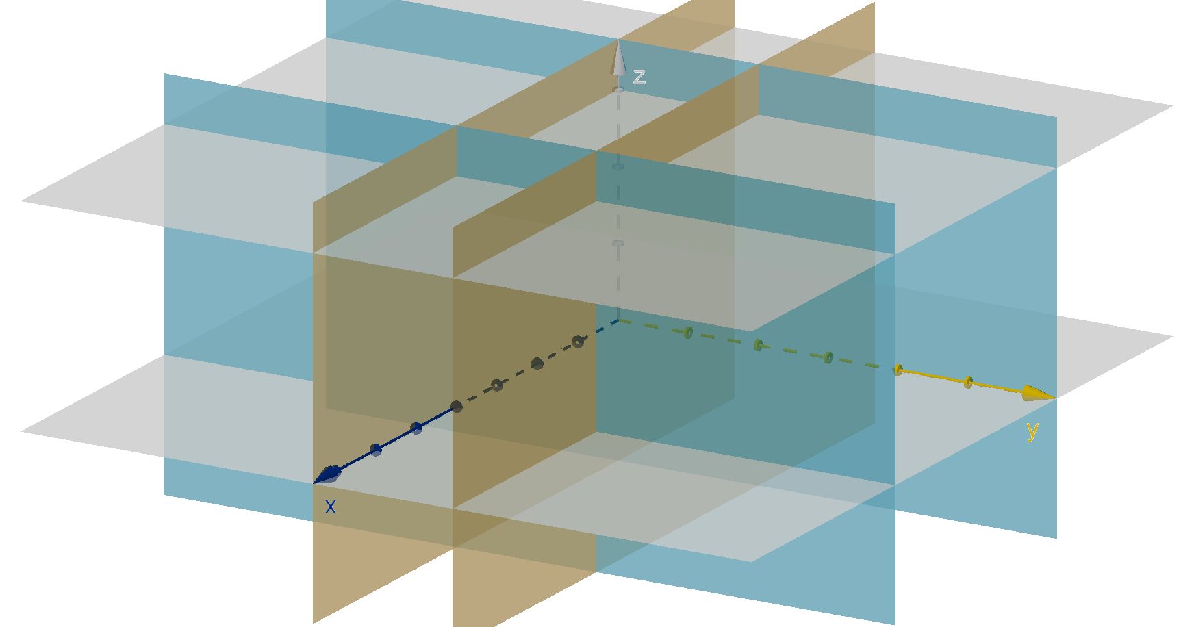
Figure: A Rectangular Prism
Solution
We will set this up as an integral of the form dzdydx. The inner integral is dz. No matter where we
are in R, we can travel in the positive z direction until we hit z = 3 or the negative z direction until we
hit z = 0. Thus the inner integral is
Z
3
0
3zy + x
2
dz.
Different choices of (x, y) will give different values of this inner integral. The points in R corresponding
to a choice of (x, y) are a vertical segment ranging from z = 0 to z = 3. These segments exist for any
(x, y) in the rectangle 0 ≤ x ≤ 4, 0 ≤ y ≤ 2. We can set up the x and y bounds over this rectangle as
we would over a normal double integral. The integrand is the dz integral above. Together we have an
iterated integral.
Z
4
0
Z
2
0
Z
3
0
3zy + x
2
dzdydx
We evaluate the inner integral, then the middle, and finally the outer.
464
Z
4
0
Z
2
0
Z
3
0
3zy + x
2
dzdydx =
Z
4
0
Z
2
0
3
2
yz
2
+ x
2
z
3
0
dydx
=
Z
4
0
Z
2
0
27
2
y + 2x
2
dydx
=
Z
4
0
27
4
y
2
+ 2x
2
y
2
0
dx
=
Z
4
0
27 + 4x
2
dx
= 27x +
4
3
x
3
4
0
= 108 +
256
3
=
580
3
Like a rectangle for double integrals, the right rectangular prism has constant bounds for triple
integrals. This is because the bounds of the inner variables remain the same, no matter what values the
outer variables take.
Question 6.4.3
How Do We Interpret Triple Integrals Geometrically?
The double integral is the volume under the graph of a two-variable function. This graph lives
in three-space. The triple integral is thus a fourth-dimensional volume “under” the graph of a three-
variable function. This graph lives in four-space and is thus more problematic to visualize. However
we can flatten the fourth dimension into three-space, much like we can flatten the three directions of
three-space onto a two-dimensional page. Such a representation loses some information, but can be a
useful heuristic. We can examine the role of each iteration in an iterated triple integral through this
construction.
Z
3
0
f(x, y, z) dz computes the area under the graph w = f(x, y, z) over each vertical segment of
the form (x, y) = (x
0
, y
0
) in the domain. It is a function of x and y.
465
Question 6.4.3
How Do We Interpret Triple Integrals Geometrically?
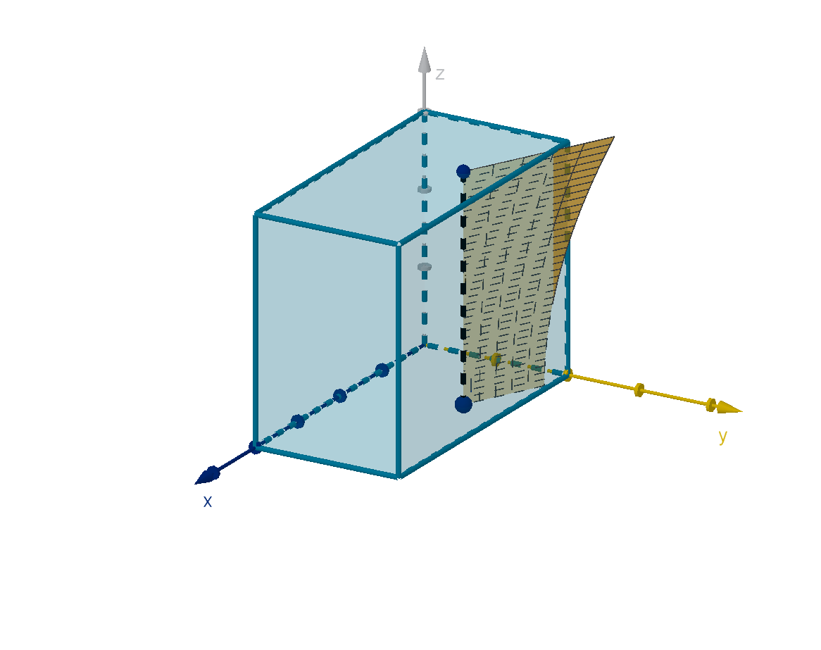
Figure:
Z
3
0
f(x, y, z) dz, represented as an area in a zw-plane
Z
2
0
Z
3
0
f(x, y, z) dzdy computes the volume under the graph w = f (x, y, z) over each x = x
0
cross-section of the domain. It is a function of x.
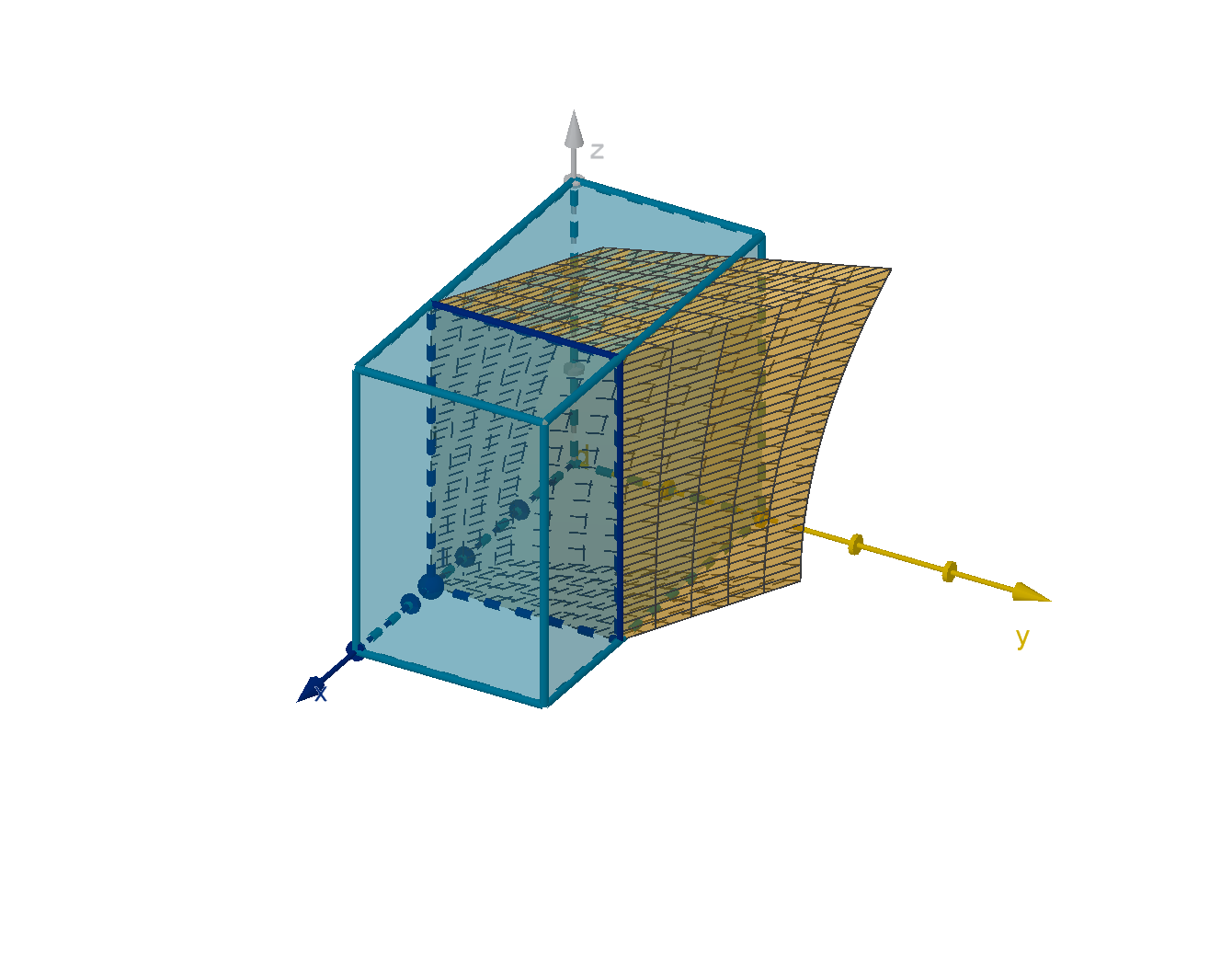
Figure:
Z
2
0
Z
3
0
f(x, y, z) dzdy, represented as a volume in yzw-space
The final integral would require us to represent a fourth-dimensional analogue of volume, which
would severely overlap in this visualization.
Application 6.4.4
Triple Integrals in Math and Science
Triple integrals have a variety of applications, largely in physics which tried to model our three-
dimensional world.
466
1 Integrating a function ρ(x, y, z), which gives the density of an object at each point, gives the total
mass of the object.
2 Integrating xρ(x, y, z), yρ(x, y, z) and zρ(x, y, z) gives the center of mass of the object.
3 Integrating a three-dimensional probability distribution over a region gives the probability that the
triple (X, Y, Z) lies in that region.
4 Integrating 1 dV over a region gives the volume of that region.
Even if we aren’t interested in physics, this connection provides us with another visual model for
integration. Density lets us visualize a triple integral without referring to a fourth (geometric) dimension.
Z
3
0
f(x, y, z) dz computes the density of
the vertical segments at each (x, y).
Z
2
0
Z
3
0
f(x, y, z) dzdy computes the den-
sity of the rectangle at each x.
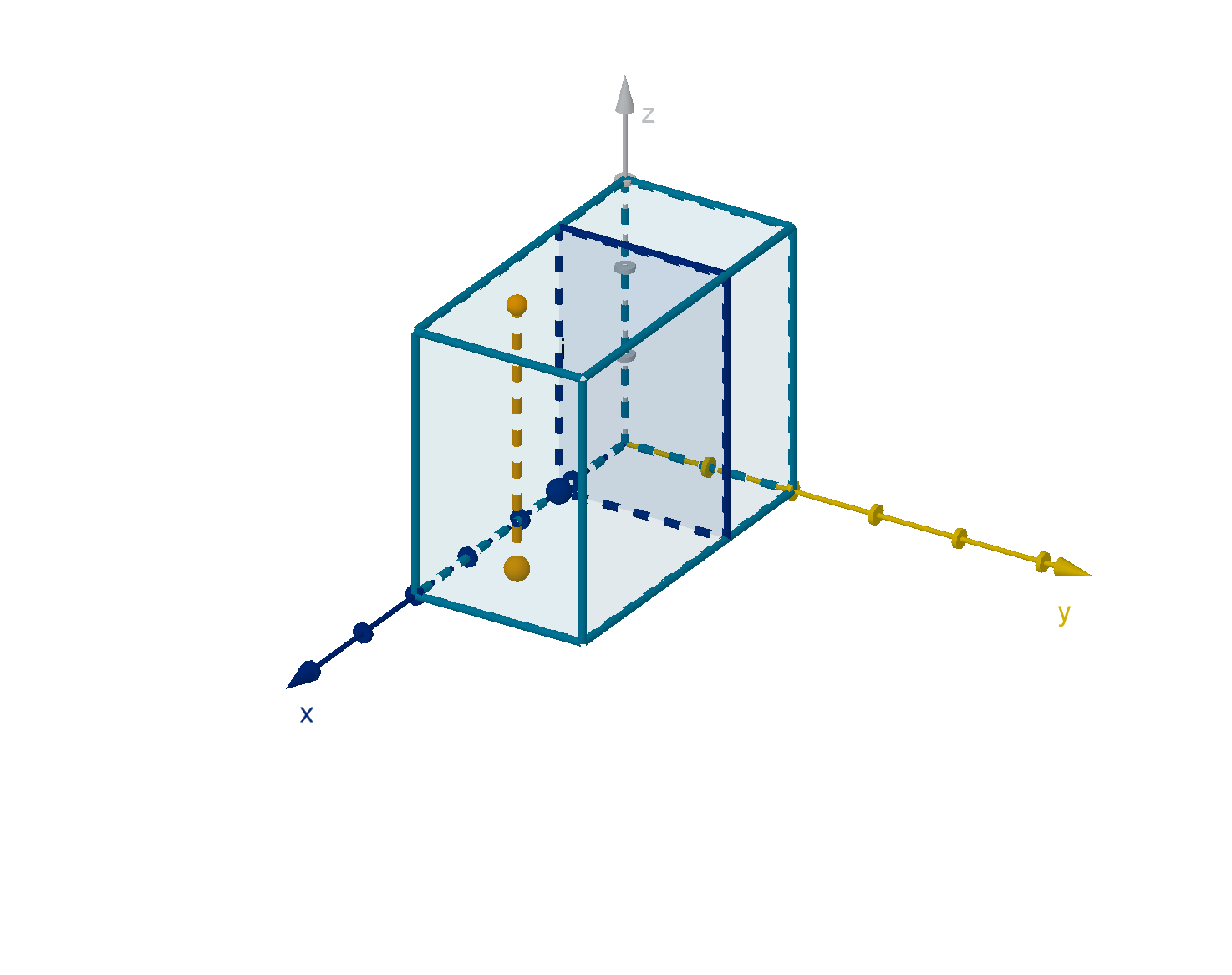
Z
4
0
Z
2
0
Z
3
0
f(x, y, z) dzdydx computes the total mass of the prism.
Remark
Technically the density at each step is a different kind of rate.
f(x, y, z) represents mass per unit of volume.
Z
3
0
f(x, y, z) dz represents mass per unit of area, since you would need all the segments above
some area to produce a volume.
Z
2
0
Z
3
0
f(x, y, z) dzdy represents mass per unit of length, since you would need to stack a segment
worth of rectangles to produce a volume.
467
Example 6.4.5
Integrating Over an Irregular Region
Let R be the region above the xy plane, below the cylinder x
2
+ z
2
= 16 and between y = 0 and
y = 3. Compute
ZZZ
R
4yz dV .
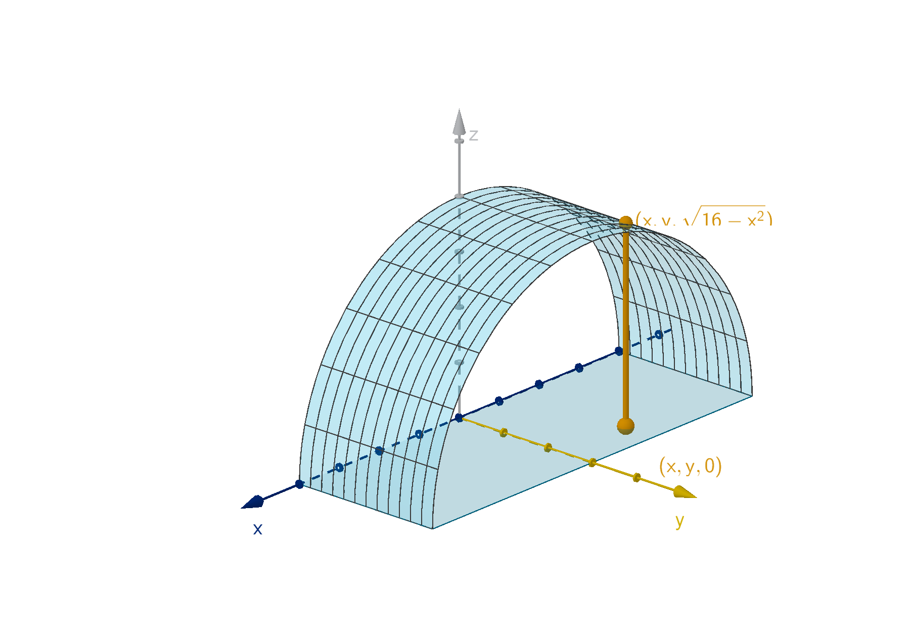
Figure: The region between x
2
+ y
2
= 16 and the xy-plane
Solution
The words “above” and “below” are useful hints here. “Above the xy-plane” indicates that for each
(x, y) the lower bound of z will be on the xy-plane, where z = 0. “Below the cylinder” indicates that
the upper bound of z will satisfy x
2
+ z
2
= 16 which solves to z = ±
√
16 − x
2
. Since these z values
are above the xy-plane, the positive branch must be the upper bound. Thus our inner integral is
Z
√
16−x
2
0
4yz dz
To complete the middle and outer bounds we consider what x and y values lie in R. The lines y = 0 and
y = 3 suggest bounds for y, but they do not enclose any region. Where else can we get information?
Since R is bounded above and below by y = 0 and above by y =
√
16 − x
2
, then it is also bounded by
where these graphs meet. We can solve for that intersection:
0 =
p
16 − x
2
0 = 16 − x
2
0 = (4 + x)(4 − x)
x = −4 or x = 4
Putting this together with the bounds we already have, we see that our x and y bounds are rectangular.
We set them up as we would in a double integral and put the inner integral as an integrand:
Z
4
−4
Z
3
0
Z
√
16−x
2
0
4yz dzdydx
468
We now turn to evaluating the integral. Having a function of x in our z-bounds should be familiar from
double integrals.
Z
4
−4
Z
3
0
Z
√
16−x
2
0
4yz dzdydx =
Z
4
−4
Z
3
0
2yz
2
√
16−x
2
0
dydx
=
Z
4
−4
Z
3
0
2y(
p
16 − x
2
)
2
dydx
=
Z
4
−4
Z
3
0
32y −2yx
2
dydx
=
Z
4
−4
16y
2
− x
2
y
2
3
0
dx
=
Z
4
−4
144 − 9x
2
dx
= 144x − 3x
3
4
−4
= 576 − 192 − (−576 + 192)
= 768
Main Idea
The following approach will produce the bounds of a region with a top surface and a bottom surface.
1 The z bounds are given by the equations z = f (x, y) and z = g(x, y) of the top and bottom
surface.
2 The intersection of the top and bottom surface can produce relevant bounds on x and y. We can
graph these, along with any given bounds involving x and y.
3 After drawing the bounded region in the xy-plane, the x and y bounds are computed as for a
double integral.
Like with double integrals, we will want to break the region into smaller pieces in some cases. In
other cases, we may want to change the order of integration.
469
Example 6.4.6
A Solid Given by Vertices
Suppose we want to integrate over T , the tetrahedron (pyramid) with vertices (0, 0, 0), (4, 0, 0),
(4, 2, 0) and (4, 0, 2). How would we set up the bounds of integration?
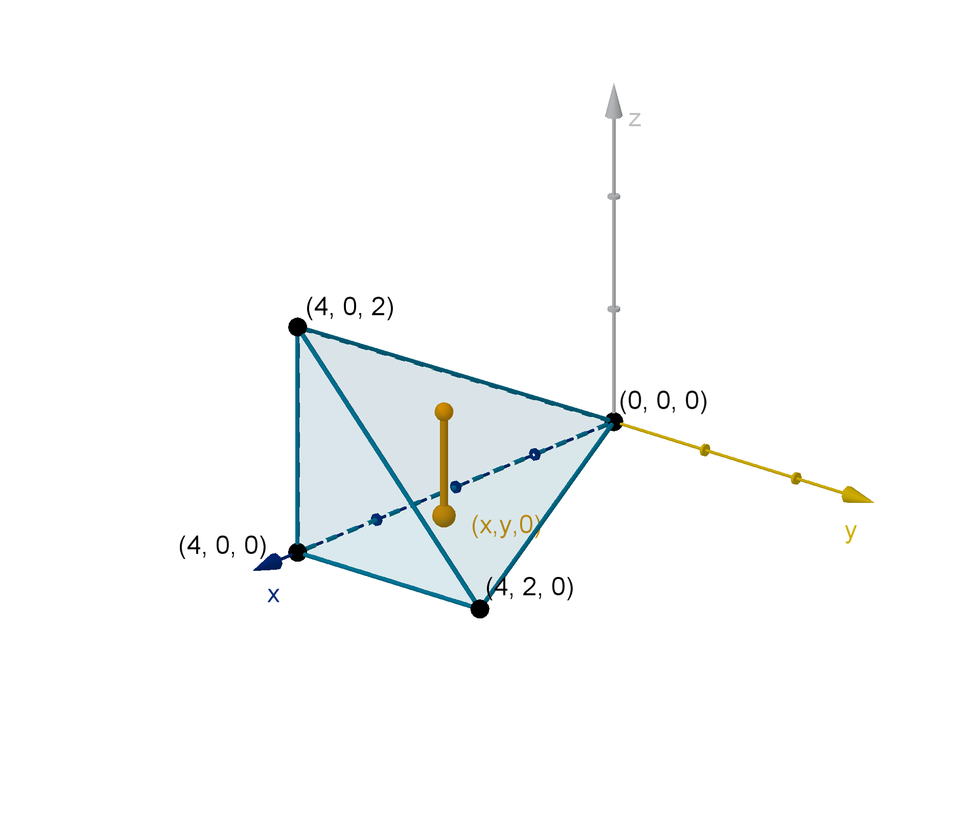
Figure: z bounds of T
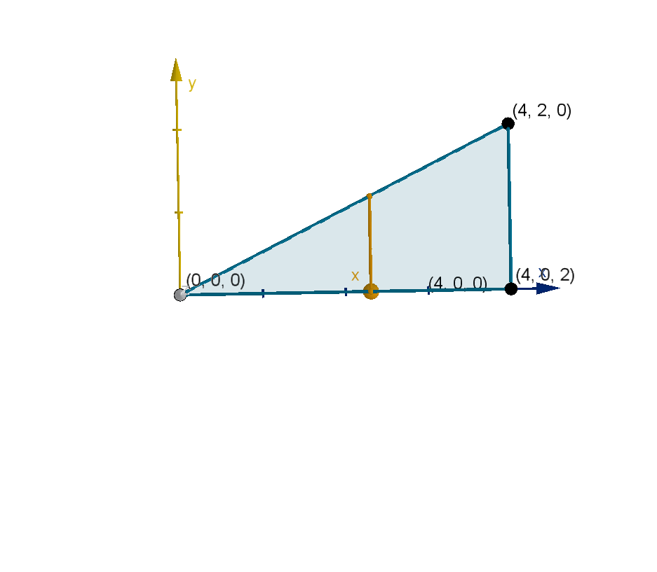
Figure: x, y bounds of T
Solution
In this case, it is helpful to draw a diagram of the tetrahedron in three-space. First we examine the inner
integral. The bounds of z are functions of (x, y). Visually, we want to imagine the vertical segments
lying in different parts of T and ask where their upper and lower endpoints lie. No matter which veritcal
segment we pick, its lower endpoint in on the xy-plane and its upper endpoint is on the triangle with
vertices (0, 0, 0), (4, 2, 0) and (4, 0, 2).
The xy-plane gives us a lower bound z = 0. The upper bound triangle also lies in a plane. Every
upper endpoint lies in this plane, so its z coordinates must satisfy the equation of that plane. This plane
has a z-intercept of 0 since (0, 0, 0) is a vertex of the triangle. We can solve for the slopes and write
the equation.
m
x
=
2 − 0
4 − 0
=
1
2
m
y
=
2 − 0
0 − 2
= −1
z =
1
2
x − 1y + 0
z =
1
2
x − y
Our inner integral is
Z
1
2
x−y
0
f(x, y, z) dz
To find the outer bounds, we ask what values of (x, y) lie in T ? Every point in T lies directly above the
triangle with vertices (0, 0, 0), (4, 2, 0) and (4, 0, 0). Thus its (x, y) coordinates match those of a point
470
in the triangle. We can draw this triangle in the xy-plane and set up the bounds of a double integral
over it. The result is
Z
4
0
Z
1
2
x
0
Z
1
2
x−y
0
f(x, y, z) dzdydx
Main Idea
In the case of a polyhedron given by vertices, we generally need to plot the vertices and draw the faces
to discern the upper and lower z bounds. The equations of these bounds are planes. We can then draw
the set of possible (x, y) in two-space and proceed as in a double integral.
Example 6.4.7
Changing the Order of Integration
Suppose D is the bounded region enclosed between the graph of y = 4x
2
+ z
2
and the plane y = 4.
Set up the bounds of the integral
ZZZ
D
f(x, y, z)dV .
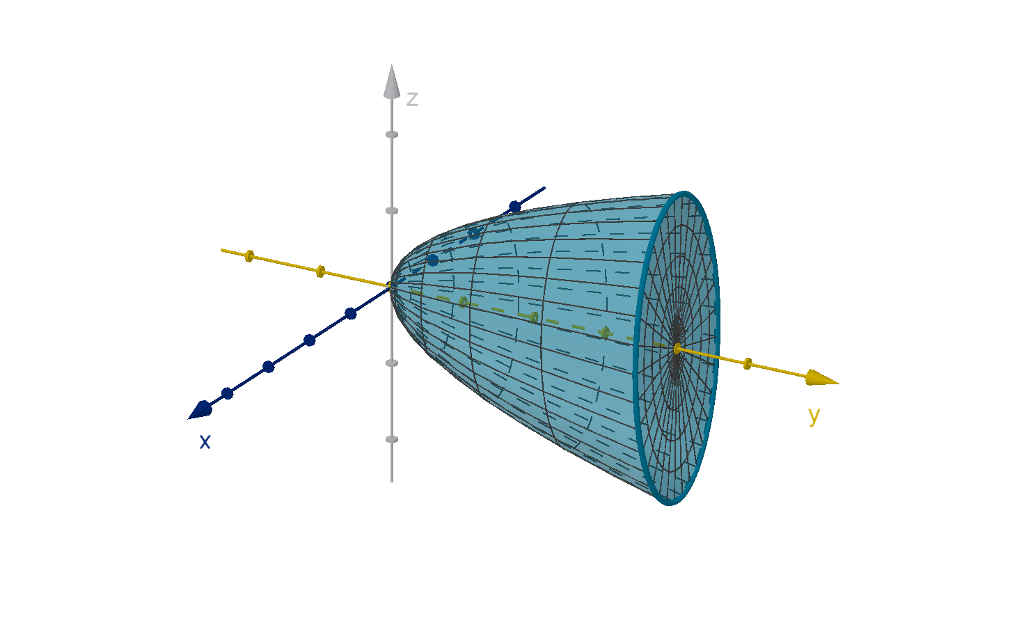
Figure: A region bounded by a paraboloid and a plane
471
Example 6.4.7
Changing the Order of Integration
Solution 1
We can begin by finding bounds for the z, the inner variable. The plane y = 4 does not have a z. z
is a free variable and thus the plane extends in the z direction, and cannot be the top or bottom of a
vertical segment. On the other hand y = 4x
2
+ z
2
solves to z = ±
p
y −4x
2
. Since this gives a plus
and a minus branch, it can provide both the upper and lower bound of z. The inner integral is
Z
√
y−4x
2
−
√
y−4x
2
f(x, y, z) dz
For xy-bounds we have equation y = 4, but this does not bound any region. We can search for additional
bounds by seeing where the top surface meets the bottom. We’ll use the fact that a square root can
only equal a negative square root if both are 0.
−
p
y −4x
2
=
p
y −4x
2
y −4x
2
= 0
y = 4x
2
We can add this parabola to a graph. We set up our xy bounds using our usual method for double
integrals. The graphs y = 4x
2
and y = 4 intersect at x = ±1. Between x = −1 and x = 1, y = 4 is
greater than y = 4x
2
. Here are the bounds.
Z
1
−1
Z
4
4x
2
Z
√
y−4x
2
−
√
y−4x
2
f(x, y, z) dzdydx
The bounds in this solution look difficult to work with. For example, in the first step, we’ll plug
p
y −4x
2
in for z in the antiderivative of f . The resulting integrand would be even more difficult
to work with. We can improve this situation somewhat by choosing a different variable for our inner
integral.
Solution 2
Since both bounds are already solved for y, we will use y as our inner variable. We can test which is
the upper and which is the lower bound with a test point, but we don’t yet know which x and z values
lie in the region. We do not have any x or z bounds that don’t involve y, so we set the y-bounds equal
to each other.
4x
2
+ z
2
= 4
We may recognize this as an ellipse. Even if we do not, we can proceed at usual for a double integral,
except that our variables are x and z. We will use z is the inner variable and solve the bound for z.
4x
2
+ z
2
= 4
z
2
= 4 − 4x
2
z = ±
p
4 − 4x
2
472
These give upper and lower bounds for z. To find x bounds, we solve for where the z-bounds intersect.
−
p
4 − 4x
2
=
p
4 − 4x
2
4 − 4x
2
= 0 a sqaure root equals its nagative only at 0
4(1 − x)(1 + x) = 0
x = −1 or x = 1
This gives us the bounds of the outer integrals:
Z
1
−1
Z
√
4−4x
2
−
√
4−4x
2
. . . dzdx
We still need a test point for the y bounds. We can choose x = 0 since that is between −1 and 1.
We can choose z = 0 since that is between −
p
4 − 4(0)
2
and
p
4 − 4(0)
2
. We plug them into both y
bounds and see that y = 4 is the upper bound.
y = (4)(0)
2
+ 0
2
vs y = 4
Our final integral is
Z
1
−1
Z
√
4−4x
2
−
√
4−4x
2
Z
4
4x
2
+z
2
f(x, y, z) dydzdx.
We still have difficult z bounds under this method, but we delay plugging them in until the second
step, which means they may cause less trouble for us.
Main Idea
When setting up a triple integral bounded by graphs, it may be more convenient to use an inner variable
that has a less complicated relationship with the bounding equations.
Question 6.4.8
When Does a Triple Integral Decompose as a Product?
The product theorem from double integrals also works here:
Theorem
If y
1
, y
2
, z
1
and z
2
are constants, then
Z
x
2
x
1
Z
y
2
y
1
Z
z
2
z
1
f(x)g(y)h(z) dzdydx
=
Z
x
2
x
1
f(x) dx
Z
y
2
y
1
g(y) dy
Z
z
2
z
1
h(z) dz
473
Question 6.4.8
When Does a Triple Integral Decompose as a Product?
Example
Along with the sum and constant multiple rules we can simplify
Z
4
0
Z
2
0
Z
3
0
3zy + x
2
dzdydx
to obtain the following:
Z
4
0
Z
2
0
Z
3
0
3zy dzdydx +
Z
4
0
Z
2
0
Z
3
0
x
2
dzdydx
=3
Z
4
0
dx
Z
2
0
y dy
Z
3
0
z dz +
Z
4
0
x
2
dx
Z
2
0
dy
Z
3
0
dz
=3 · 4
Z
2
0
y dy
Z
3
0
z dz + 2 · 3
Z
4
0
x
2
dx
Section 6.4
Exercises
Summary Questions
Q1
What does Fubini’s theorem say about integrals with dV ?
Q2
How is density used to understand triple integrals. Why wasn’t it necessary or appropriate for
double integrals?
Q3
How do you find the bounds of the inner variable in a triple integral?
Q4
How to you find the bounds of the other two variables?
474
6.4.1
Q5
Suppose we want to approximate
Z
3
0
Z
10
2
Z
2
−2
f(x, y, z) dzdydx by subdividing the domain of
integration into 12 sub-prisms of equal volume. What will V be?
Q6
Let R be a cube of side length 4, with edges parallel to the x-, y- and z-axes, and with vertices
(0, 0, 0) and (4, 4, 4). Suppose we want to approximate
ZZZ
R
xyzdV using a subdivsion of R
into 8 identical cubes.
a
What will V be?
b
What test points would you use to make your approximation as large as possible.
c
Produce the smallest possible approximation using this subdivision.
6.4.2
Q7
Is
Z
4
0
Z
7
0
Z
2
0
f(x, y, z) dzdydx =
Z
7
0
Z
2
0
Z
4
0
f(x, y, z) dzdydx? Explain.
Q8
Set up the bounds of integration of a function f(x, y, z) over the a general prism
P = {(x, y, z) : x
0
≤ x ≤ x
1
, y
0
≤ y ≤ y
1
, z
0
≤ z ≤ z
1
}
Q9
Evaluate
Z
2
0
Z
2
0
Z
3
0
(x + y)z dzdydx.
Q10
Evaluate
Z
5
0
Z
11
0
Z
1
−1
ye
2x+z
dzdydx.
475
Section 6.4
Exercises
6.4.3
Q11
In a triple integral, the inner integral
Z
z
1
z
0
f(x, y, z) dz is a function of x and y, while
Z
y
1
y
0
Z
z
1
z
0
f(x, y, z) dzdy
is a function of only x.
a
Explain why this occurs algebraically.
b
Explain why this makes sense given the context of an iterated triple integral.
Q12
In each of the following questions, assume x, y, z, and w are the variables of four-space.
a
What is the dimension of the set of points that satisfy x = x
0
?
b
What is the dimension of the set of points that satisfy both x = x
0
and y = y
0
?
Q13
Give the area of the x = 4 and y = 1 cross-section of the region “under” the graph of w = x+ye
z
and “above” the prism
P = {(x, y, z) : 0 ≤ x ≤ 6, 0 ≤ y ≤ 4, 0 ≤ z ≤ 3}
Q14
Give the volume of the x = 2 cross-section of the region “under” the graph of w =
z
2
√
13−x
2
y
and “above” the prism
P = {(x, y, z) : 0 ≤ x ≤ 3, 1 ≤ y ≤ 2, −3 ≤ z ≤ 3}
6.4.4
Q15
A prism of length ℓ, width w and height h can be defined by the inequalities
0 ≤ x ≤ ℓ
0 ≤ y ≤ w
0 ≤ z ≤ h
Set up a triple integral to compute the volume of this prism. Verify that the value of this integral
matches the well-known volume formula, V = ℓwh.
476
Q16
Denser matter tends to sink to the bottom of a container. After sitting undisturbed for several
days, the density of a soil sample in the box
P = {(x, y, z) : 0 ≤ x ≤ 5, 0 ≤ y ≤ 4, 0 ≤ z ≤ 2}
is given by ρ(x, y, z) = e
−z/10
. Find the total mass of the soil in the box.
Q17
Xavier, Yolanda and Zoe’s respective arrival times (in hours after noon) at a restaurant are given
by joint random variables X, Y and Z. The joint density function of X, Y and Z is
f
X,Y,Z
(x, y, z) =
(
12
11
(1 − x
2
yz) if 0 ≤ x ≤ 1, 0 ≤ y ≤ 1, 0 ≤ z ≤ 1
0 otherwise
Compute the probability that they all arive by 12 : 15.
Q18
Random variables X, Y and Z are uniform if their density function has the form
f
X,Y,Z
(x, y, z) =
(
1
V
if (x, y, z) is in R
0 otherwise
where V is the volume of R. If X, Y and Z are uniform on
R = {(x, y, z) : 0 ≤ x ≤ 10, 0 ≤ y ≤ 10, 0 ≤ z ≤ 10},
compute P (X ≤ 4 and Z ≥ 3).
6.4.5
Q19
Let R be the region given by x
2
+ y
2
+ z
2
≤ 25.
a
Describe R geometrically.
b
Set up the bounds of integration for
ZZZ
R
f(x, y, z) dV .
c
If we plug in the function f(x, y, z) = 1 do you happen to know the value of this integral?
Q20
Cheng is integrating over R, the region given by x
2
+ y
2
+ z
2
≤ 25. He gives the following setup.
Is this valid?
Z
√
25−y
2
−z
2
−
√
25−y
2
−z
2
Z
√
25−x
2
−z
2
−
√
25−x
2
−z
2
Z
√
25−x
2
−y
2
−
√
25−x
2
−y
2
f(x, y, z) dzdydx
477
Section 6.4
Exercises
Q21
Consider the domain
D : {(x, y, z) : y ≥ 0, y ≤ −x, z ≥ 9, z ≤ 25 − x
2
− y
2
}
a
Set up the bounds of
RRR
D
x dV . Do not evaluate.
b
Do you expect the integral in
a
to be positive, negative, or zero? In a sentence or two,
explain how you know without computing it.
Q22
Let R = {(x, y, z) : z ≤ 2x − y, z ≥ 0, y ≥ x
2
}. Compute
ZZZ
R
xz dV.
Q23
Let R be the region enclosed by the graphs z = x
2
+ y
2
and 2y −z = 0. Set up the bounds for
RRR
R
(y −1) dV . Do not evaluate.
Q24
Set up a triple integral that will compute the volume enclosed by the planes x = 0, x = 5, y = 0,
z = 2y and z = 6. Do not evaluate.
Q25
Let R be the region enclosed by z = x
2
, z = 16, y = 2 and y = 6. Set up and evaluate
ZZZ
R
x + z dV .
Q26
Let R be the region enclosed by y =
√
25 − x
2
, z = 6 − y and z =
√
y. Set up the bounds of
RRR
R
g(x, y, z)dV .
6.4.6
Q27
Let P be a square pyramid with vertices (0, 0, 0), (2, 0, 0), (2, 2, 0), (0, 2, 0) and (0, 0, 4).
a
Explain why it might not be a good idea to use z as the inner variable when setting up the
bounds of
ZZZ
P
f(x, y, z) dV .
b
Set up the bounds using a different inner variable.
478
Q28
Set up the bounds of integration of
ZZZ
T
f(x, y, z) dV , where T is a tetrahedron with vertices
(0, 0, 0), (8, 0, 0), (0, 6, 0) and (0, 0, 3).
6.4.7
Q29
Let R be the region over the first quadrant enclosed by y = x
2
, x = 0, z = 0 and z = 4 − y.
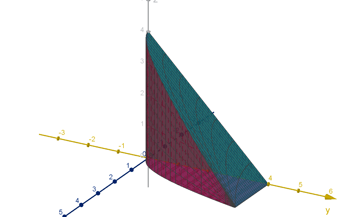
Set up the integral
ZZZ
R
f(x, y, z) dV
a
with z as the inner variable
b
with y as the inner variable
c
with x as the inner variable
Q30
Let R be the region enclosed by the paraboloid x = 3 −y
2
− z
2
and the plane y =
1
2
x.
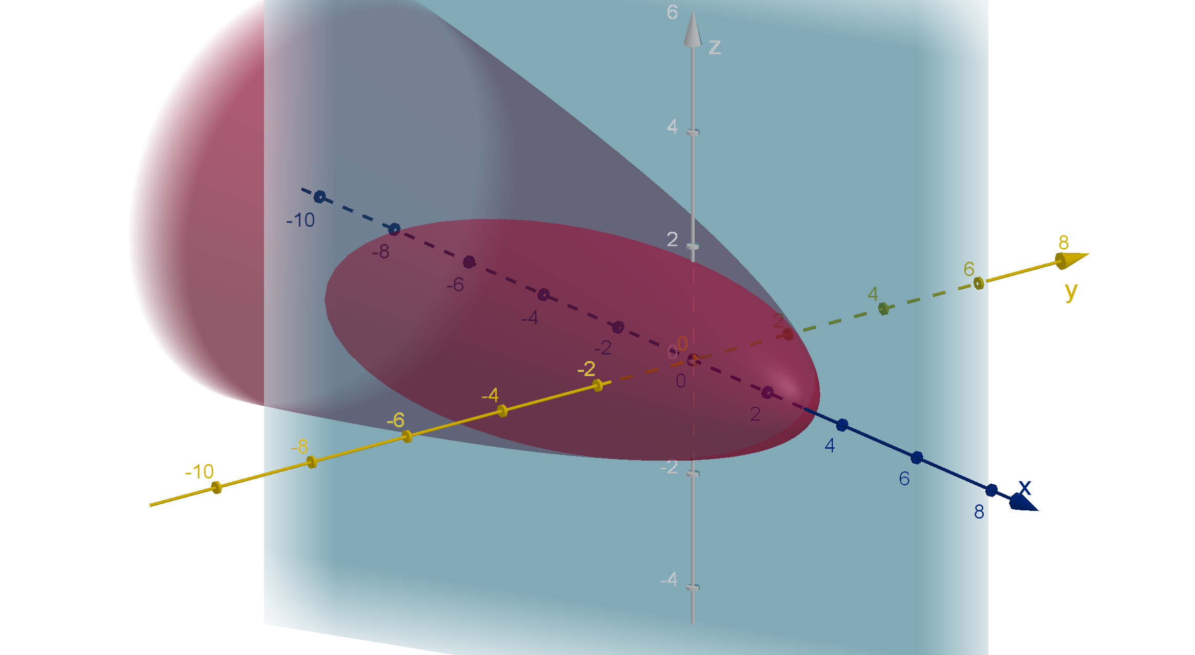
a
Set up the integral
RRR
R
f(x, y, z) dV with z as the inner variable.
479
Section 6.4
Exercises
b
Set up the integral
RRR
R
f(x, y, z) dV with x as the inner variable.
c
Explain why it would be difficult to set up
RRR
R
f(x, y, z) dV with y as the inner variable.
Q31
Let P be the prism whose base has vertices (0, 0, 0), (0, 5, 0) and (0, 0, −2) and whose height is
4 units in the direction of the positive x axis. Set up a triple integral
RRR
P
g(x, y, z) dV in three
different ways, using three different inner variables.
Q32
Let P be the trapezoidal prism with vertices (0, 0, 0), (0, 6, 0), (0, 4, 2), (0, 0, 2), (5, 0, 0), (5, 6, 0),
(5, 4, 2), and (5, 0, 2). Set up the bounds of integration of
ZZZ
P
h(x, y, z) dV without writing
it as a sum or difference of multiple integrals.
Q33
Consider the tetrahedron T whose vertices are (0, 0, 0), (0, 0, 4), (0, 6, 3), (2, 6, 3). Which vari-
able(s) could you use as the inner variable of a triple integral over T without having to break the
domain into two or more pieces.
Q34
Set up (but do not evaluate) one or more integrals of f (x, y, z) over the region
R = {(x, y, z) : z ≥ 0, x ≥ y
2
+ z
2
, x + 2z ≤ 8}
Use dxdydz as your order of integration.
Q35
Rewrite the integral
Z
1
0
Z
x
x
2
Z
x−y
0
f(x, y, z) dzdydx as an integral with the differential dxdzdy.
Q36
Rewrite the integral
Z
2
0
Z
2
2−x
Z
4−x
2
0
f(x, y, z) dzdydx as an integral with the differential dxdzdy.
6.4.8
Q37
Use product and sum rules to decompose
Z
4
3
Z
8
0
Z
1
−1
y
2
sin x − e
y+z
dzdydx into an expression
containing only single integrals.
Q38
Let S = {(x, y, z) : x
2
+ y
2
+ z
2
≤ 25}. Explain why
ZZZ
S
x
3
y
4
cos πz dV cannot be
decomposed as a product.
480
Synthesis & Extension
Q39
Consider the domain
D : {(x, y, z) : x − 16 ≤ y ≤ 2, x
2
+ y
2
≤ z ≤ x
2
+ x + 4}
a
Set up the bounds of
RRR
D
xyz dV . You may use one or more integrals to do so. Do not
evaluate.
b
Does the function f (x, y, z) = xyz have a maximum value on D? Justify your answer with
a theorem, and verify that the theorem does or does not apply.
Q40
Let S be the region above z = 0 and below the graph z = f(x, y) over the rectangle
R = {(x, y) : a ≤ x ≤ b, c ≤ y ≤ d}.
a
Write the volume of S as a double integral.
b
Write the volume of S as a triple integral.
c
Show that if you evaluated your answer to
b
, your answer to
a
would be one of the step
of this computation.
Q41
Suppose that R is the solid obtained by rotating the region under y = f(x) from x = a to x = b
around the x-axis. Write a triple integral that computes the volume of R.
481