Chapter 5
Vectors in Calculus
This chapter introduces vectors and their applications to calculus. We will use them to compute direc-
tional derivatives, to differentiate compositions of functions, and to find minimum and maximum values
of a function.
Contents
5.1 Vectors . . . . . . . . . . . . . . . . . . . . . . . . . . . . . . . . . . . . . . 306
5.2 The Dot Product . . . . . . . . . . . . . . . . . . . . . . . . . . . . . . . . 321
5.3 Normal Equations of Planes . . . . . . . . . . . . . . . . . . . . . . . . . . . 330
5.4 The Gradient Vector . . . . . . . . . . . . . . . . . . . . . . . . . . . . . . . 342
5.5 The Chain Rule . . . . . . . . . . . . . . . . . . . . . . . . . . . . . . . . . 359
5.6 Maximum and Minimum Values . . . . . . . . . . . . . . . . . . . . . . . . 375
5.7 Lagrange Multipliers . . . . . . . . . . . . . . . . . . . . . . . . . . . . . . . 393
Section 5.1
Vectors
Goals:
1 Distinguish vectors from scalars (real numbers) and points.
2 Add and subtract vectors, multiply by scalars.
3 Express real world vectors in terms of their components.
Calculus is the study of change. We defined the partial derivative to be instantaneous rate of change
of a multi-variable function when one variable changed but the other stayed constant. If we want to
describe a more complicated change, we will need new notations and vocabulary to describe them. We
will need vectors.
Question 5.1.1
What is a Vector?
A vector is a way of describing a change in position in n-space. To keep things simple, we’ll start
with vectors in the plane. We need two pieces of information to identify a vector.
Definition
A vector in 2-space consists of a magnitude (length) and a direction. Two vectors with the same
magnitude and the same direction are equal.
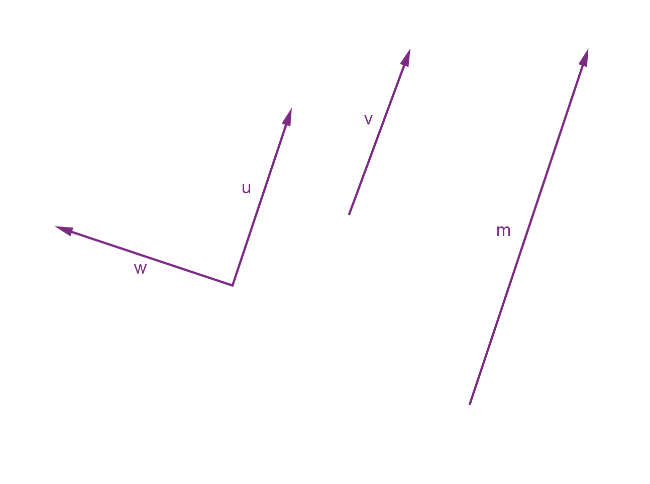
Example
Here are four vectors in 2-space (the plane) represented by arrows. Two of these vectors are equal.
Here are some vectors
3 miles south
306
The force that a magnetic field applies to a charged particle
The velocity of an airplane
Here are some non-vectors
17
The mass of an automobile
3:15 PM
Atlanta, GA
Question 5.1.2
How Do We Denote Vectors?
When defining a new type of object, we need to agree on a notation. This allows us to communicate
clearly which vector we are referring to. One way of denoting a vector is by its endpoints.
Endpoint Notation
The vector v from point A to point B can be represented by the notation
−−→
AB.
A is the initial point and B is the terminal point.
How does this notation interact with the idea of equal vectors?
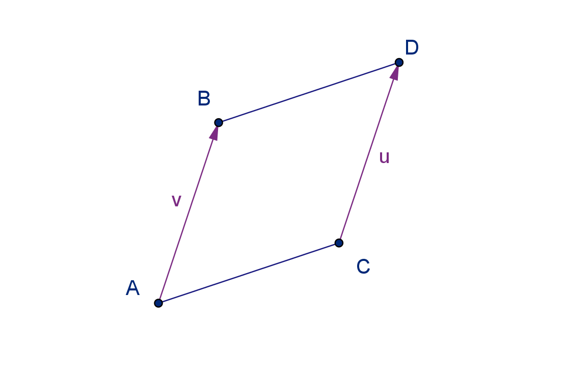
Theorem
−−→
AB =
−−→
CD if and only if ABDC is a parallelogram (perhaps a squished one).
The plane has a coordinate system. We can take advantage of this to produce a more quantitative
notation for vectors.
307
Question 5.1.2
How Do We Denote Vectors?
Coordinate Notation
We can represent a vector in the Cartesian plane by the x and y components of its displacement. If
A = (2, 3) and B = (5, 1), then
−−→
AB increases x by 5 − 2 = 3 and y by 1 − 3 = −2. We can represent
−−→
AB = ⟨3, −2⟩
Figure: The x and y components of a vector
We can use coordinate notation to quickly test whether two vectors are equal.
Theorem
v = u if and only if their coordinate representations match in each component.
We can also measure slope using the coordinate notation. For the vector v = ⟨a, b⟩:
b represents the displacement in the y-direction (rise).
a represents the displacement in the x-direction (run).
The slope of v is
rise
run
=
b
a
.
Vectors are not points, but their coordinate notations look awfully similar. We can connect them
more formally. Every point in a Cartesian coordinate system has a position vector, which gives the
displacement of that point from the origin. The components of the vector are the coordinates of the
point.
308
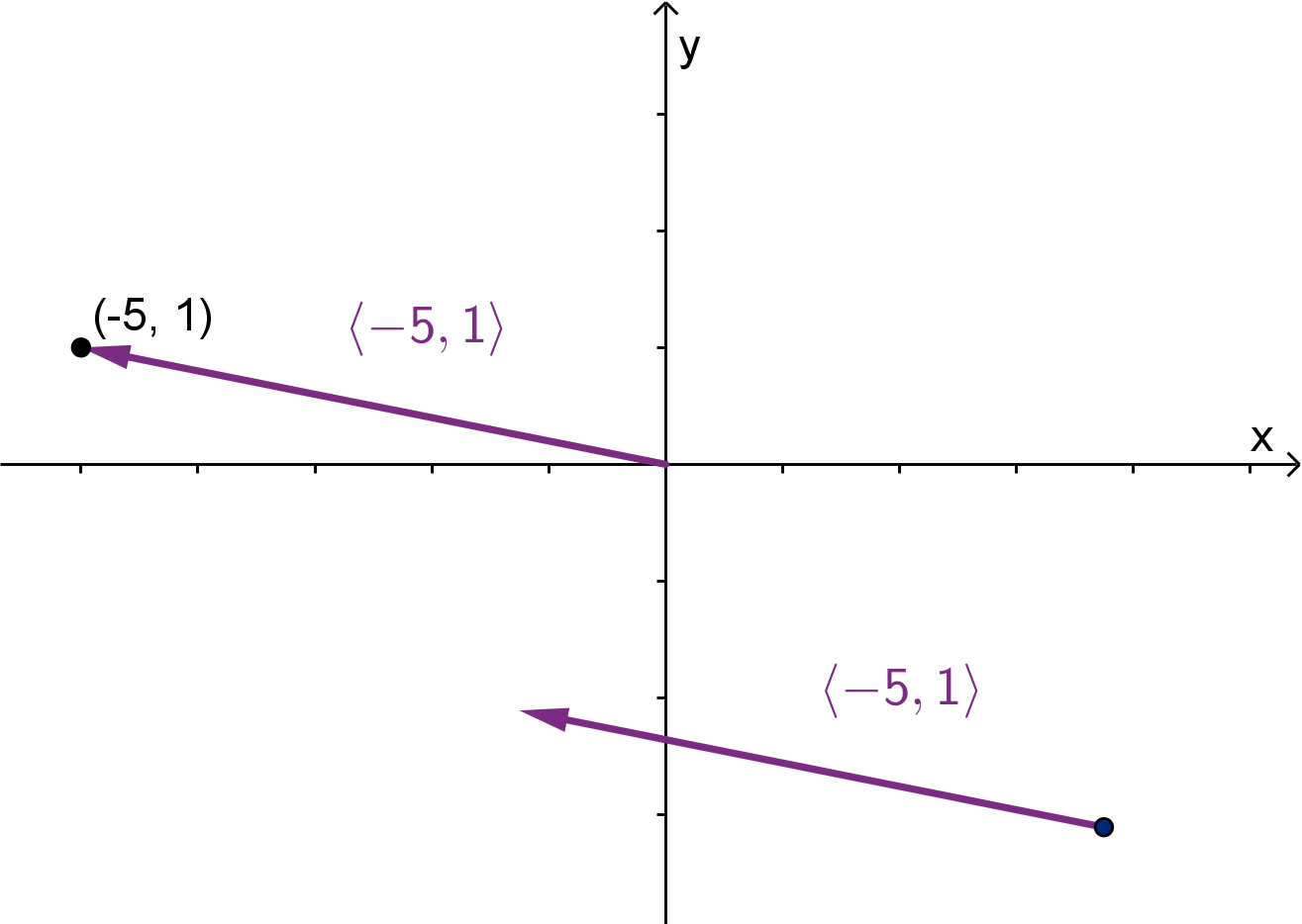
Figure: There is only one point equal to (−5, 1), but there are many vectors equal to ⟨−5, 1⟩.
Question 5.1.3
What Arithmetic Can We Perform with Vectors?
Unlike locations (points), displacements (vectors) can be added and multiplied. This arithmetic
allows unlocks a variety of computations and measurements, specifically it will allow us to do calculus.
Since we have multiple ways of representing vectors, we will want to understand how to perform these
operations with each of those representations.
309
Question 5.1.3
What Arithmetic Can We Perform with Vectors?
Vector Sums
The sum of two vectors v + u is calculated by positioning v and u head to tail. The sum is the vector
from the initial point of one to the terminal point of the other. In coordinate notation, we just add each
component numerically.
⟨ 1, 3⟩
+⟨ 3, −1⟩
⟨ 4, 2⟩
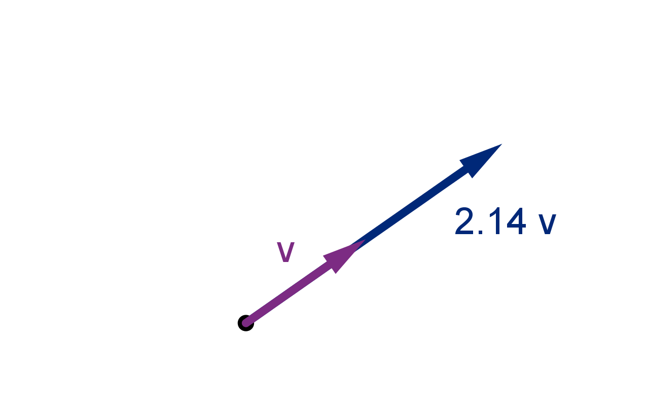
Scalar Multiples
Given a number (called a scalar) λ and a vector v we can produce the scalar multiple λv, which is the
vector in the same direction as v but λ times as long.
If λ is negative then λv extends in the opposite di-
rection. Either way, we say λv is parallel to v.
In coordinates scalar multiplication is distributed to each component. For example:
2.5 ⟨6, 4⟩ = ⟨15, 10⟩
310
Example 5.1.4
Performing Vector Arithmetic
Given diagrams of two vectors u and v, how would we calculate
1
2
u + v?
What if we are instead given the components u = ⟨a, b⟩ and v = ⟨c, d⟩?
Solution
After drawing a random u and a random v, we draw
1
2
u in the same direction as u but is half as long.
We place it head to tail with v, and
1
2
u + v completes the triangle.
In coordinates the computation is as follows.
1
2
u + v =
1
2
⟨a, b⟩+ ⟨c, d⟩
=
1
2
a,
1
2
b
+ ⟨c, d⟩
=
1
2
a + c,
1
2
b + d
311
Question 5.1.5
What Is Standard Basis Notation?
Vector arithmetic gives us another notation that takes advantage of our algebraic intuition. We can
represent any vector in the plane as a sum of scalar multiples of the following standard basis vectors.
Standard Basis Vectors
The emphstandard basis vectors in R
2
are
i = ⟨1, 0⟩
j = ⟨0, 1⟩
For example, the vector ⟨3, −5⟩ can be written as 3
i − 5
j. You can check yourself that the sum on
the right gives the correct vector.
Question 5.1.6
How Do We Measure the Length of a Vector?
A vector consists of two pieces of information: magnitude and direction. How do we measure these?
Length is the distance between the endpoints. We already have a method for measuring distance in the
plane.
Definition
The length or magnitude of a vector is calculated using the distance formula and notated |v|. If
v = a
i + b
j, then
|v| =
p
a
2
+ b
2
312
Example 5.1.7
The Length of a Vector
If v = ⟨3, −5⟩ calculate |v|
Solution
|v| =
p
3
2
+ (−5)
2
=
√
34
Definition
A unit vector is a vector of length 1. Given a vector v the scalar multiple
1
|v|
v
is a unit vector in the same direction as v.
Question 5.1.8
How Do We Measure the Direction of a Vector?
Direction cannot be described as clearly as length. How do we even measure it? A partial answer is
to measure the difference in direction between two vectors.
Angles are a good way of comparing directions. In general, two vectors will not intersect to form an
angle, so we use the following definition:
Definition
The angle between two vectors is the angle they make when they are placed so their initial points are
the same.
If they make a right angle, we call them orthogonal. If they make an angle of 0 or π, they are
parallel.
313
Question 5.1.9
How Do We Denote Vectors in Higher Dimensions?
Higher dimensional vectors represent displacements in higher dimensional spaces. We can call a
vector in n-space an n-vector. We can still denote and n-vector by its endpoints. We can also denote
it in coordinate notation, but we need more components.
Example
If A = (2, 4, 1) and B = (5, −1, 3) then
−−→
AB = ⟨3, −5, 2⟩.
In three space, we add another standard basis vector
k.
Standard basis for 3-vectors
i = ⟨1, 0, 0⟩
j = ⟨0, 1, 0⟩
k = ⟨0, 0, 1⟩
Example
⟨3, −5, 2⟩ = 3
i − 5
j + 2
k
Higher dimensions still have a standard basis, but at this point the naming conventions are less
standard. {e
1
, e
2
, e
3
, . . . , e
n
} is common for n-vectors.
Length of a Vector
The length of an n-vector derives from the distance formula in n-space.
|⟨a
1
, a
2
, a
3
, . . . , a
n
⟩| =
q
a
2
1
+ a
2
2
+ a
2
3
+ ···+ a
2
n
We might be concerned that direction becomes an even more difficult concept to work with as the
dimension increases. However, angles are a valid a way of comparing directions any dimension (though
they may be more difficult to compute).
314
Angles Between Vectors
Any two vectors with the same initial point lie in a plane. Their angle is a two-dimensional measurement.
However there is no good way to measure clockwise in 3 or more dimensions. The angle between
two vectors is never negative, nor more than π.
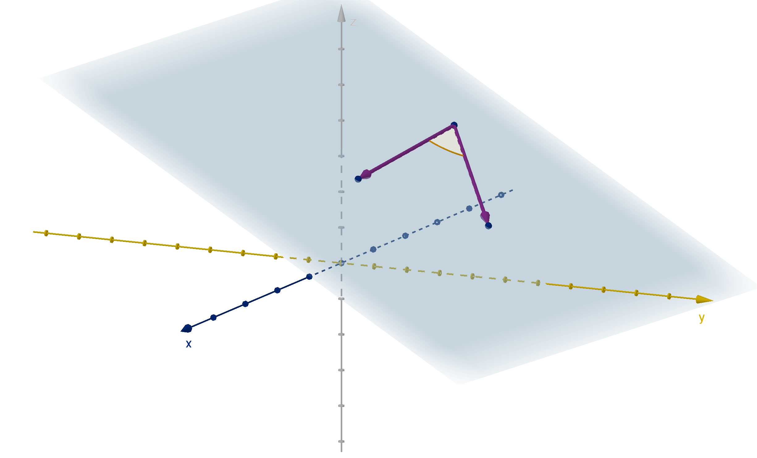
Figure: Two 3-vectors with a common initial point, the plane that contains them, and the angle
between them
Section 5.1
Exercises
Summary Questions
Q1
How is a vector similar to a point? To a number?
Q2
How is a vector different from a point? From a number?
Q3
How can you tell if two vectors point in the same direction? Opposite directions?
Q4
If u and v are position vectors of the points P and Q, how are u and v related to
−−→
P Q?
315
Section 5.1
Exercises
5.1.1
Q5
Which of the following are vectors?
i. The reading on a speedometer.
ii. The intersection of two lines.
iii. Five miles toward Atlanta.
iv. The length of a string.
v. The velocity of a projectile.
Q6
Which of the following are vectors?
i. The displacement of a key on a keyboard, when pressed.
ii. The speed of light.
iii. The center of the earth.
iv. The force applied by a rocket engine.
v. The mass of five hippopotamuses.
Q7
If
−−→
AB =
−→
AC, what does that tell us about the points B and C? Explain.
Q8
If
−−→
AB =
−−→
BA, what does that tell us about the points A and B? Explain.
5.1.2
Q9
If A = (8, 7, 11) and B = (2, 3, 15) write the vector
−−→
AB
a
in terms of its components
b
in standard basis notation
Q10
If P = (−2, 3, 5) and Q = (−2, 0, −4) write the vector
−−→
P Q
a
in terms of its components
b
in standard basis notation
Q11
What is the slope of the vector −4
i + 10
j?
Q12
Give three different vectors of slope
3
7
.
316
Q13
Suppose two different vectors have the equal slopes. How are they related?
Q14
Given a number m, give two different vectors with slope m.
5.1.3
Q15
Let u be a vector. How are the magnitude and direction of u and 2u related?
Q16
How is the direction and magnitude of u related to the direction and magnitude of −u?
Q17
Given diagrams of two vectors u and v, how would we draw u −v? What it its significance?
Q18
If u is a vector and
2u = u, what does that tell us about u? Explain.
Q19
If u =
−−→
AB, v =
−→
AC, and
1
2
u +
1
2
v =
−−→
AD, where is D?
Q20
If u =
−−→
AB, v =
−→
AC, and
1
5
u +
4
5
v =
−−→
AD, where is D?
5.1.4
Q21
Let u = 4
i + 3
j and v = 5
i − 2
j. Compute u + v.
Q22
Let w = ⟨5, −1⟩ and v = ⟨12, 10⟩. Compute w −v.
Q23
For Lindsey to get from her house to Sam’s house, she travels 5mi north and 3mi west. To
get to Russel’s house, she travels 2mi due south. What displacement would get her from Sam’s
house to Russel’s house?
Q24
One can get from Atlanta to Decatur by travelling 8km east and 2km north. To get from
Decatur to Covington, one can travel 43km east and 20km south. Describe how to get directly
from Atlanta to Covington.
Q25
Using the diagram below, describe each vector in terms of u and v using vector addition and
scalar multiplication. Use the fact that ACDB and ACBE are parallelograms.
317
Section 5.1
Exercises
a
−−→
EB
b
−−→
CG
c
−−→
BC
d
−→
AF
e
−−→
GB
Q26
Using the diagram below, describe each vector in terms of u and v using vector addition and
scalar multiplication. Use the fact that ACBD is a parallelogram, and the marked segments are
congruent.
a
−−→
BD
b
−→
EA
c
−−→
DC
d
−−→
BG
e
−→
AG
f
−−→
CF
5.1.5
Q27
Write ⟨5, 2⟩ in standard basis notation.
Q28
For any numbers a and b, use the definition of
i and
j to show that a
i + b
j = ⟨a, b⟩.
318
5.1.6
Q29
Compute the length of u = ⟨−5, 12⟩.
Q30
Given a nonzero vector u, many vectors of length 5 are parallel to u? Explain.
Q31
Find a unit vector in the direction of 3
i −
j.
Q32
Find a unit vector in the direction of ⟨12, −16⟩.
5.1.7
Q33
If u and v are vectors in R
2
whose components are all positive, what is the largest possible angle
between u and v?
Q34
Explain the difference between the terms “perpendicular” and “orthogonal.”
Q35
Suppose two vectors do not have the same inital point, but when we represent them by arrows,
the arrows happen to cross. Is the angle made in the crossing equal to the angle between the
vectors (as we defined it)?
Q36
Describe all the vectors that make an angle of
π
4
with v = −
j.
5.1.8
Q37
If u = ⟨2, 0, 3⟩ and v = ⟨5, 6, 0⟩, compute 3u − 4v.
Q38
If a = 10
i − 25
k and
b = 8
i − 4
j + 10
k, compute
3
5
a +
1
2
b.
Q39
Compute the magnitude of v = 2
i − 7
j + 6
k.
Q40
Compute two unit vectors parallel to v = ⟨4, −4, 2⟩.
319
Section 5.1
Exercises
Q41 a
How many different (nonequal) unit vectors are orthogonal to a given vector in R
2
? How
are they related to each other?
b
How many different (nonequal) unit vectors are orthogonal to a given vector in R
3
? How
are they related to each other?
Q42
Let u and v be non-parallel vectors in R
3
. How many unit vectors in R
3
are orthogonal to both
u and v?
Synthesis and Extension
Q43
Is the vector v = 2
i + 3
j + 8
k parallel to the plane p whose slope-intercept equation is z =
x + 2y − 7?
Q44
For a two-variable function f (x, y), f
x
(x
0
, y
0
) is the slope of the line tangent to z = f(x, y) at
(x
0
, y
0
, f(x
0
, y
0
)) in the x-direction. Write a vector v that is parallel to this line.
Q45
If u =
−−→
AB and v =
−→
AC, show that for any scalar t, tu + (1 − t)v = AD where D is a point on
the line through B and C.
Q46
If u, v and w are position vectors of the three vertices A, B and C of a triangle, then
1
3
(u+v + w)
is the position vector of K, the center of mass of the triangle. Verify this by showing that K lies
on the line between A and the midpoint of the side BC.
Q47
Suppose we become interested in studying vectors of infinite dimension (yes this is something
mathematicians actually do).
a
Explain what trouble we might run computing the length of the vector ⟨1, 1, 1, 1, 1, . . .⟩.
b
What would the length of the vector ⟨1,
1
2
,
1
4
,
1
8
,
1
16
, . . .⟩ be?
320
Section 5.2
The Dot Product
Goals:
1 Calculate the dot product of two vectors.
2 Determine the geometric relationship between two vectors based on their dot product.
3 Calculate vector and scalar projections of one vector onto another.
The arithmetic of vectors appears to have room for expansion. While we can add and subtract
vectors, we only defined how to multiply them by scalars, not by other vectors. There are in fact
products of two vectors. The simplest and most useful is the dot product. The dot product takes two
n-vectors and outputs a single number. Despite this apparent loss of information, the dot product is
the key tool in computing the angle between vectors, the work done by a force, or the illumination in a
digital scene.
Question 5.2.1
What Is the Dot Product?
Definition
The dot product of two vectors is a number.
For two dimensional vectors v = ⟨v
1
, v
2
⟩ and u = ⟨u
1
, u
2
⟩ we define
v ·u = v
1
u
1
+ v
2
u
2
For three dimensional vectors v = ⟨v
1
, v
2
, v
3
⟩ and u = ⟨u
1
, u
2
, u
3
⟩ we define
v ·u = v
1
u
1
+ v
2
u
2
+ v
3
u
3
This pattern can be extended to any dimension.
Example 5.2.2
Computing a Dot Product
a
Calculate ⟨2, 3, −1⟩· ⟨4, 1, 5⟩
b
Calculate (−2
i + 4
k) · (
i + 2
j −
k)
321
Example 5.2.2
Computing a Dot Product
Solution
a
⟨2, 3, −1⟩·⟨4, 1, 5⟩ = (2)(4) + (3)(1) + (−1)(5) = 6
b
(−2
i + 4
k) · (
i + 2
j −
k) = (−2)(1) + (0)(2) + (4)(−1) = −6
Question 5.2.3
What Are the Algebraic Properties of the Dot Product?
Theorem
The following algebraic properties hold for any vectors u, v and w and scalars m and n.
Commutative u ·v = v ·u
Distributive u · (v + w) = u ·v + u · w
Associative mu · nv = mn(u ·v)
Question 5.2.4
What Is the Geometric Significance of the Dot Product?
u · v encodes key information about the magnitude and direction of u and v. This geometric
relationship can be derived from the algebraic properties we’ve established. We begin with the idea that
u · u = |u|
2
. This doesn’t tell us the value of every dot product, but we can extend the reasoning to
any pair of parallel vectors.
322
Theorem
If u and v are parallel then
u ·v =
(
|u||v| if u and v have the same direction
−|u||v| if u and v have opposite directions
Since u and v are parallel, we can write v = mu for some scalar m. v is m times as long as u. Both
lengths are positive, so this means if m > 0 then |v| = m|u|, but if m < 0, then |v| = −m|u|
u ·v = u · (mu)
= mu · u
= m|u|
2
= |u|m|u|
=
(
|u||v| if u and v have the same direction
−|u||v| if u and v have opposite directions
We can establish the dot product in another special case: when the vectors are orthogonal.
Theorem
If u and v are orthogonal then
u ·v = 0.
In this case, we place u and v head to tail and draw u + v. Since u and v make a right angle, these
three vectors make a right triangle. The Pythagorean theorem applies to the lengths of the vectors.
Figure: Orthogonal vectors and their sum making a right triangle
|u + v|
2
= |u|
2
+ |v|
2
(Pythagorean theorem)
(u + v) · (u + v) = u · u + v ·v
u · u + u ·v + v · u + v ·v = u · u + v ·v (distributive property)
u ·v + v · u = 0
2u ·v = 0 (commutative property)
u ·v = 0
323
Question 5.2.4
What Is the Geometric Significance of the Dot Product?
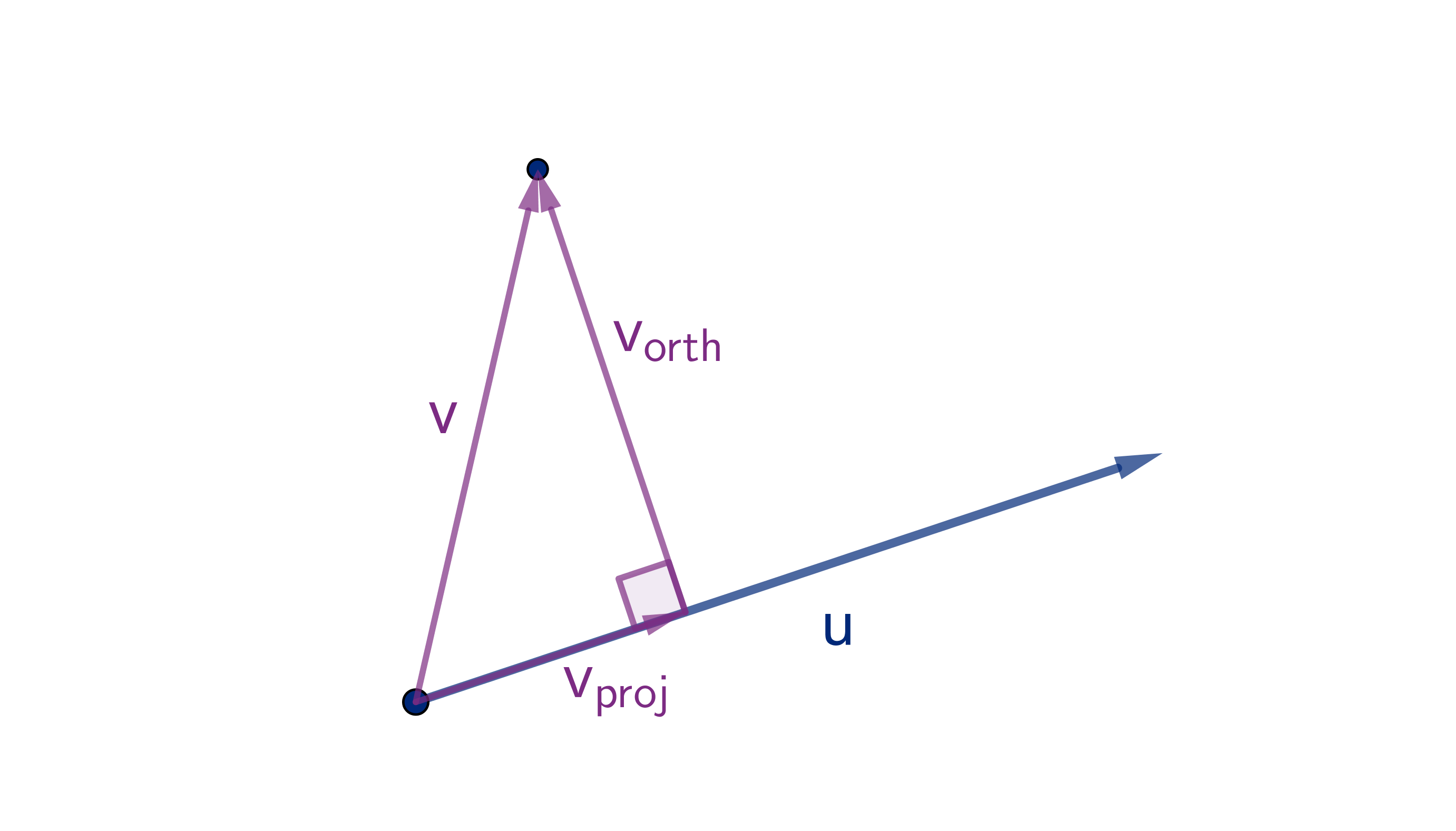
Two vectors need not be parallel or orthogonal, but given vectors u and v we can always write
v = v
proj
+ v
orth
. We choose v
proj
to be parallel to u and v
orth
to be orthogonal to u.
The properties of the dot product tell us that
u ·v =u · (v
proj
+ v
orth
)
= ± |u||v
proj
| + 0
Definition
The number
u ·v
|u|
is called the scalar projec-
tion of v onto u.
The scalar projection is equal to the length of v
proj
if v
proj
is in the same direction as u. Otherwise,
it is the negative of the length.
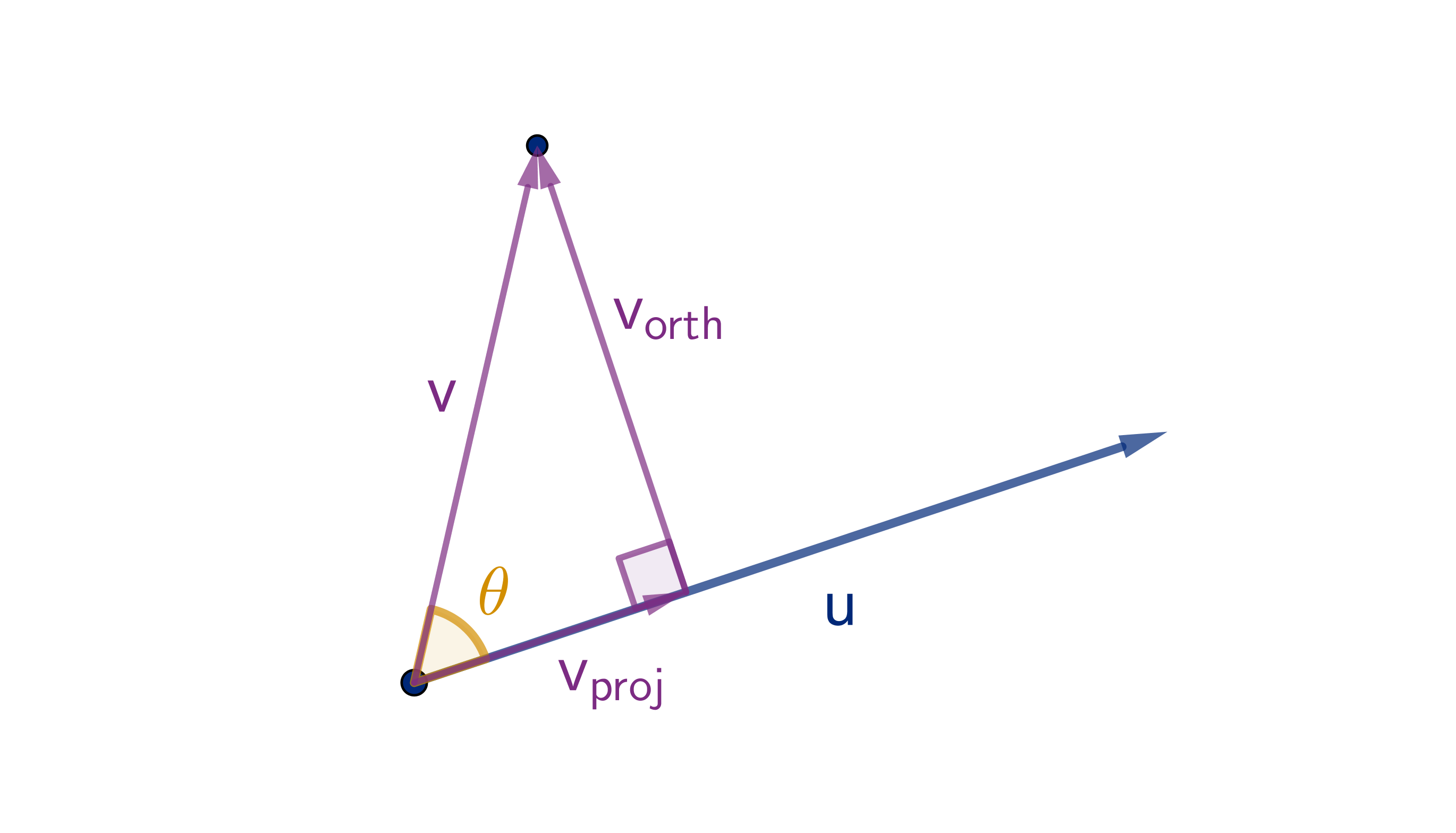
Theorem
Let u and v have the same initial point and meet at angle θ. The following formula holds in any
dimension:
u ·v = |u||v|cos θ
Recall that cos θ is
positive when θ < π/2
negative when θ > π/2
zero when θ = π/2.
So the sign of u · v tells us whether θ is
acute, obtuse or right.
Example 5.2.5
Using the Cosine Formula
What is the angle between ⟨1, 0, 1⟩ and ⟨1, 1, 0⟩?
324
Solution
We’ll apply the cosine formula, compute all of the components besides θ and solve.
⟨1, 0, 1⟩·⟨1, 1, 0⟩ = |⟨1, 0, 1⟩||⟨1, 1, 0⟩|cos θ
(1)(1) + (0)(1) + (1)(0) =
p
1
2
+ 0
2
+ 1
2
p
1
2
+ 1
2
+ 0
2
cos θ
1 =
√
2
√
2 cos θ
1
2
= cos θ
cos
−1
1
2
= θ
π
3
= θ
We can verify this by noting that these vectors are diagonals in a unit cube. We could connect them
with a third diagonal to make an equilateral triangle. We may recall that an equilateral triangle has
angles of
π
3
.
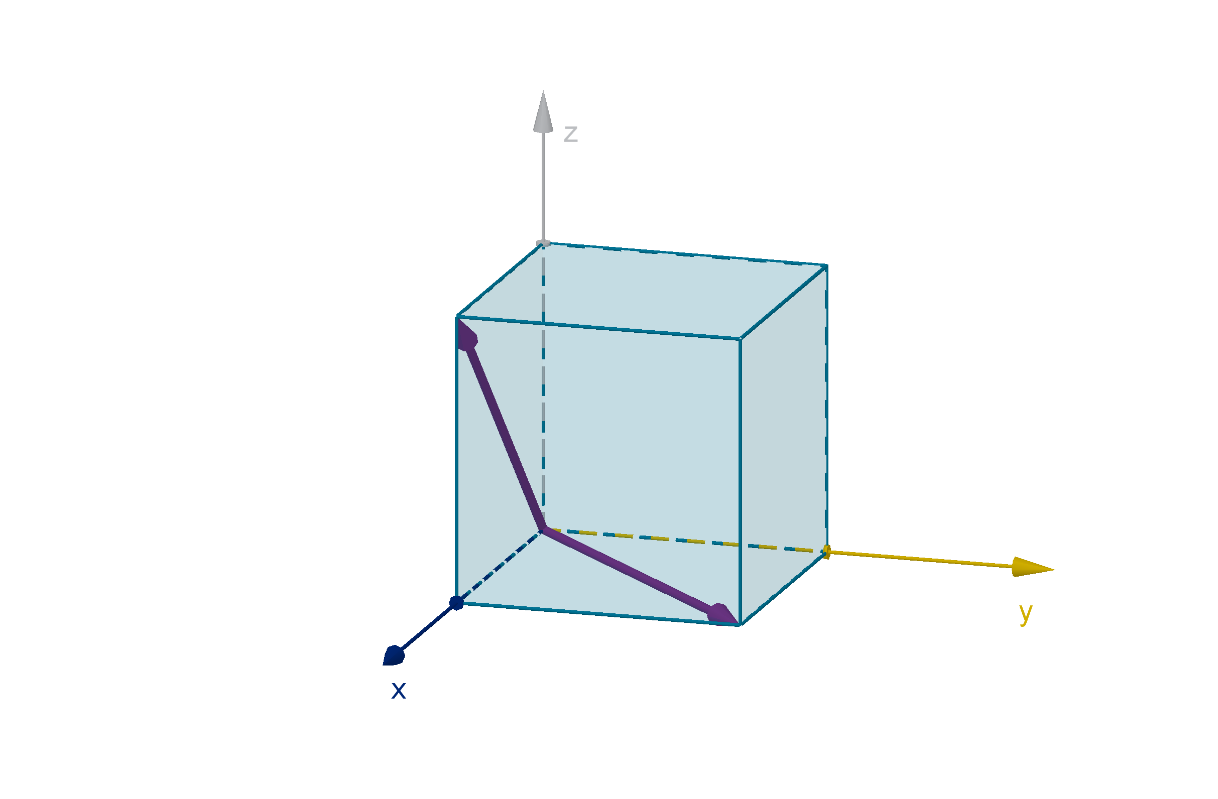
Figure: Two vectors in a unit cube
Application 5.2.6
Work
In physics, we say a force works on an object if it moves the object in the direction of the force.
Given a force F and a displacement s, the formula for work is:
W = F s
325
Application 5.2.6
Work
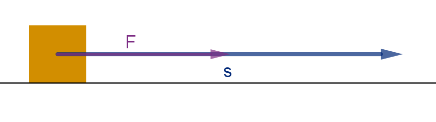
In higher dimensions, displacement and force are vectors. If the force and the displacement are not
in the same direction, then only
F
proj
contributes to work.
W =
F
proj
·s =
F ·s
Section 5.2
Exercises
Summary Questions
Q1
What algebraic properties does a dot product share with real number multiplication?
Q2
What is the significance of the dot product of two parallel vectors?
Q3
How is the angle between two vectors related to their dot product?
Q4
What is a scalar projection, and how do you compute it?
326
5.2.1
Q5
What do v ·
i and v ·
j measure about v?
Q6
Elaine computes u·v and gets ⟨15, 4⟩. How can you tell that Elaine got the wrong answer without
even knowing what u and v are?
5.2.2
Q7
Compute the following dot products.
a
⟨4, 5⟩· ⟨−1, −2⟩
b
(5
i + 6
j) · (
i − 2
j)
c
⟨2, 4, −10⟩·⟨0, −1, −2⟩
Q8
Compute the following dot products.
a
⟨4, 5⟩· ⟨−1, −2⟩
b
(5
i + 6
j) · (
i − 2
j)
c
(2
i − 3
k) · (7
j −
k)
5.2.3
Q9
Let u = ⟨2, 3⟩, v = ⟨4, −1⟩ and w = ⟨−5, 2⟩.
a
Compute u · u and u ·v and u · w.
b
Compute v · u. How does it compare to u ·v?
327
Section 5.2
Exercises
c
How is u · u related to |u|?
d
Compute 3u and 3v then take their dot product. How is it related to u ·v?
e
Compute v + w then compute u · (v + w). How is it related to u ·v and u · w?
f
Why do you think we call this operation a “dot product” and not a “dot sum?”
g
If you wanted to prove that relationships your noticed in
b
-
e
work for all possible vectors,
how would you do that?
Q10
Expand the parentheses 2u · (3v − w).
Q11
Expand the parentheses (a − 3
b) · (5c + 2
d).
Q12
Factor a ·a + 6a ·
b + 9
b ·
b.
5.2.4
Q13
Suppose we know that u and v are parallel, that |v| = 4 and that u ·v = −28.
a
What is the length of u?
b
What can you say about the directions of u and v?
Q14
If |u| = 12, |v| = 9, and u ·v = 0, what is the magnitude of the vector w = u + v?
Q15
If |u| = 5 and u ·v = 15, what are the possible values of |v|?
Q16
If |u| = 6 and |v| = 10 what are the greatest and least possible values of u ·v?
Q17
Let v = 7
i − 2
j +
k, what unit vector u produces the largest possible dot product u ·v?
Q18
Argue that u ·v cannot be any larger than |u||v|.
328
5.2.5
Q19
Compute the angle between ⟨6, 1, 4⟩ and ⟨7, 0, 2⟩.
Q20
Compute the angle between ⟨0, 3, −5⟩ and ⟨3, −4, 3⟩.
Q21
Let A be the vertex of a cube. Let B the a vertex closest to A and C be the vertex farthest from
A. Compute the angle between
−−→
AB and
−→
AC.
Q22
Let A be the vertex of a cube, and B and C be any two other points on the cube. Use a dot
product to explain why the angle between
−−→
AB and
−→
AC cannot be larger than
π
2
. (Hint, put A
at (0, 0, 0).)
Synthesis and Extension
Q23
How could you use the dot product to determine whether two vectors are parallel? How does this
compare with the methods we already have?
Q24
Use dot products to find at least one vector that is orthogonal to both ⟨5, −1, 2⟩ and ⟨4, 4, 1⟩
Q25
“Think of a vector v” says Raphael, “tell me its dot product with the vector of my choice, and
I’ll tell you what your vector was.”
a
Is there any mathematical way to make such a trick work? Explain.
b
How many dot products would you need to ask for to uniquely identify an unknown vector?
What dot products would you ask for?
329
Section 5.3
Normal Equations of Planes
Goals:
1 Give equations of planes in both vector and normal forms.
2 Use normal vectors to measure the distance to a plane.
Question 5.3.1
What is a Normal Vector to a Plane?
In algebra, you learned the normal equation of a line: e.g. 2x + 3y −12 = 0. Why is it called this?
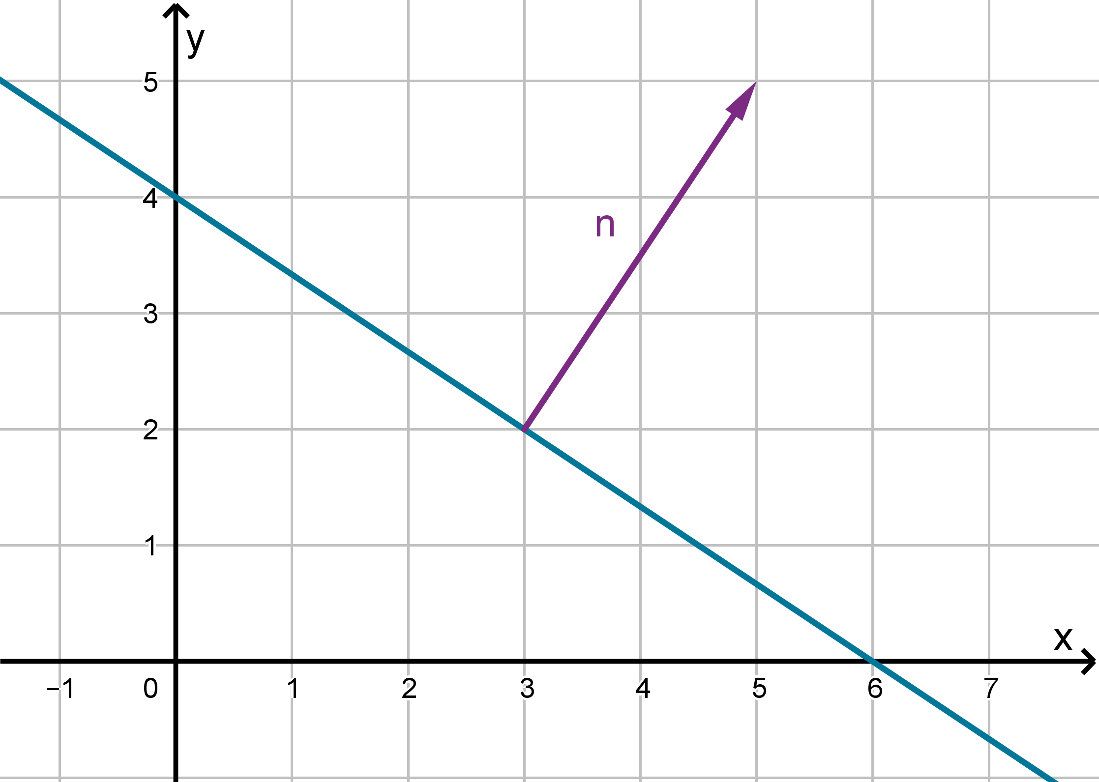
Figure: A line and one of its normal vectors
The vector ⟨2, 3⟩ is a normal vector to the line, meaning it is orthogonal to any vector contained in
the line. We can extend this definition to planes in 3-space. A normal vector to a plane is orthogonal
to every vector in the plane.
Theorem
In three-dimensional space, every plane has normal vectors. They are all parallel to each other.
330
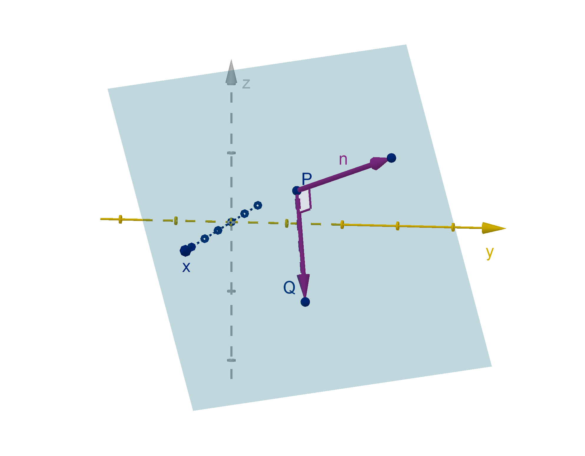
Figure: A plane, its normal vector n, and a vector
−−→
P Q in the plane
This gives us an avenue to test whether a point Q lies on the plane or not. If
−−→
P Q is orthogonal to
n, then Q lies on the plane. If
−−→
P Q and n make a different angle, then Q is not on the plane.
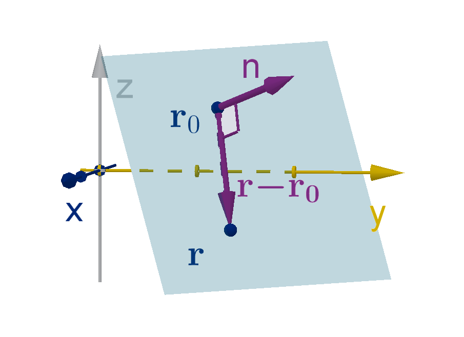
We’d like to rewrite this relationship terms of the coordinates of Q. If r
0
is the position vector of
P and r is the position vector of Q, then
−−→
P Q = r −r
0
. The dot product gives us a simple test to see
whether this vector is orthogonal to n.
Theorem
If r
0
= ⟨x
0
, y
0
, z
0
⟩ describes an known point on a plane, and n = ⟨a, b, c⟩ is a normal vector. Then
the normal equation of the plane is
(r −r
0
) ·n = 0
or
a(x − x
0
) + b(y − y
0
) + c(z − z
0
) = 0
Notice that since x
0
, y
0
and z
0
are constants, we can distribute and collect them into a single term:
d.
ax + by + cz − ax
0
− by
0
− cz
0
= 0
ax + by + cz + d = 0
This reasoning works in any dimension to define a set of points whose displacement from a known
point is orthogonal to some normal vector.
331
Question 5.3.1
What is a Normal Vector to a Plane?
Example
a(x − x
0
) + b(y − y
0
) = 0 defines a line.
a(x − x
0
) + b(y − y
0
) + c(z − z
0
) = 0 defines a plane.
a
1
(x
1
− c
1
) + a
2
(x
2
− c
2
) + ··· + a
n
(x
n
− c
n
) = 0 defines a hyperplane.
Example 5.3.2
Computing a Normal Vector
Find the normal equation of the plane with intercepts (4, 0, 0), (0, 3, 0) and (0, 0, 8). Compute a
normal vector.
Solution
The normal equation of a plane has the form ax + by + cz + d = 0. Each of these points must satisfy
this equation. We will plug them in and see what they tell me about the coefficients.
a(4) + b(0) + c(0) + d = 0 4a + d = 0
d = −4a
a(0) + b(3) + c(0) + d = 0 3b + d = 0
d = −3b
a(0) + b(0) + c(8) + d = 0 8c + d = 0
d = −8c
There are infinitely many solutions to this system of equations. This makes sense, because there are
infinitely many normal vectors to a plane. Different choices of d give n’s that are scalar multiples of
each other. A convenient choice for d is −24, but any nonzero value will work. d = −24 gives
6x + 8y + 3z − 24 = 0
The normal vector is ⟨6, 8, 3⟩.
332
Synthesis 5.3.3
Using the Normal Vector to Compute Distance
Consider the line 2x + 3y − 12 = 0.
This is the line with normal vector n = ⟨2, 3⟩ and known point P = (3, 2).
Example
Let P
1
= (7, 2) and P
2
= (4, 0).
1 Draw the vectors
−−→
P P
1
and
−−→
P P
2
.
2 If you didn’t have a picture, how could you use the values of n ·
−−→
P P
1
and n ·
−−→
P P
2
to determine
which side of the line P
1
and P
2
lie on?
Solution
Since n is a normal vector, its angle with any vector in the line is
π
2
. The vectors on the same side of
the line as n make an acute angle with n. The vectors on the far side make an obtuse angle. Thus
when n ·
−−→
P P
i
< 0, P
i
lies on the far side of the line from n. When n ·
−−→
P P
i
> 0, P
i
lies on the same side
as n.
We can get more detailed information than just the sign of the dot product. We can actually compute
a distance.
333
Synthesis 5.3.3
Using the Normal Vector to Compute Distance
Theorem
Given a line, plane, or hyperplane with normal equation L(x
1
, . . . , x
k
) = 0 and corresponding normal
vector n, the signed distance from the hyperplane to the point Q = (q
1
, . . . , q
k
) is
L(q
1
, . . . , q
k
)
n
.
Let P be a known point on the hyperplane. The scalar projection of
−−→
P Q onto n is equal to the
signed distance from the hyperplane to Q.
Figure: The scalar projection of
−−→
P Q onto the normal vector of a line
Distance =
−−→
P Q · n
|n|
(formula for scalar projection)
=
L(q
1
, . . . , q
k
)
|n|
(normal equation of the plane)
This formula is especially powerful because we do not need to know a point on the hyperplane. The
equations
a(x − x
0
) + b(y − y
0
) + c(z − z
0
) = 0
ax + by + cz + d = 0
are equivalent, and correspond to the same normal vector. We can use whichever one we happen to
have in our signed distance formula.
334
Example 5.3.4
The Distance from a Plane
Compute the geometric distance from the origin to the plane 6x + 8y + 3z − 24 = 0.
Solution
n = ⟨6, 8, 3⟩. The signed distance from the plane to the origin is
L(0, 0, 0)
|n|
=
(6)(0) + (8)(0) + (3)(0) − 24
√
36 + 64 + 9
= −
24
√
109
Geometric distance cannot be negative, so it is
24
√
109
.
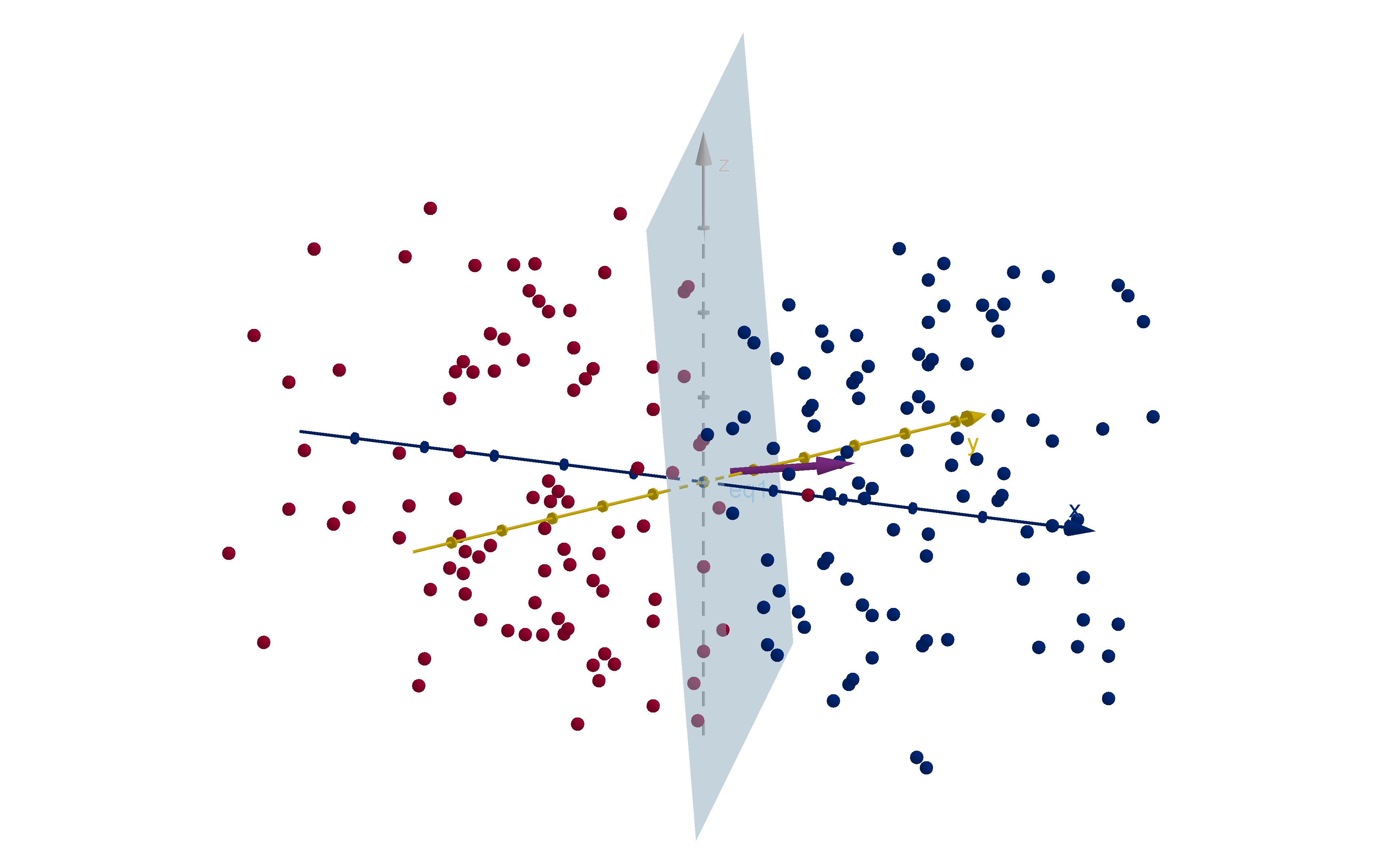
Application 5.3.5
Support Vector Machines
One type of machine learning involves training a computer to distinguish between two states. For
example, a computer might be trained to distinguish between a cancerous tumor and a benign one.
To do this the computer is given a large set of cases. Each case is measured by numerical data, such
as:
The size of the tumor
The location of the tumor
The age of the patient
Results of blood tests
The brightness of each pixel in a CT scan or MRI
Each data type is a dimension, and each case is a point in a (probably very high) dimensional space.
The computer would like a simple test to divide these cases into cancerous and benign. The test will
be which side of a hyperplane they lie on. It is unlikely that any such hyperplane exists initially, so the
computer attempts a sequence of transformations of the data until they are separated by a hyperplane
with some degree of reliability.
335
Application 5.3.5
Support Vector Machines
Section 5.3
Exercises
Summary Questions
Q1
What information do you need in order to write the normal equation of a plane?
Q2
How are the normal vectors of a plane related to each other?
Q3
What is the significance of the coefficients in the normal equation of a plane?
Q4
How do we compute the signed distance from a point to a plane?
336
5.3.1
Q5
Is v = ⟨8, −3, −10⟩ parallel to the plane 6x + 6y + 3z + 11 = 0? Explain.
Q6
Is v = 9
i − 15
j + 6
k normal to the plane −6x + 10y − 4z + 23 = 0? Explain.
Q7
Name a normal vector to the following planes:
i. 3x − 8y + 10z − 4 = 0
ii. z − 2 = 4(x + 7) − 5(y + 1)
Q8
Suppose that n is a normal vector to 6x −3y + 2z −4 = 0, that happens to also be a unit vector.
Give all possible values of n.
Q9
Write a normal equation of a plane parallel to 7x − 11y + 8z + 15 = 0 that passes through the
origin.
Q10
Write a normal equation of a plane parallel to 10x − 11y + z + 20 = 0 that passes through
(2, 3, 5).
Q11
Given that the plane ax + by + cz + d = 0 passes through the origin, what can you say about a,
b, c, and d?
Q12
Given that plane ax + by + cz + d = 0 contains the x-axis, what can you say about a, b, c, and
d?
Q13
Are the planes 4x + 6y + 8z + 15 = 0 and 10x + 15y + 20z − 7 = 0 parallel? Explain how you
know.
Q14
Suppose we know the planes 12x + 18y + 6z − 15 = 0 and ax + by + 4z + d = 0 are parallel.
What can you say about the values of a, b and d?
Q15
The equations 3x −y + 4z + 10 = 0 and −6x + 2y −8z + k = 0 describe the same plane. What
is the value of k?
Q16
Consider the plane with normal equation 7x + y − 2z = 5.
a
Give two other normal equations of this plane.
b
What are the normal vectors corresponding to the orginal equation and your two equations
in
a
?
337
Section 5.3
Exercises
c
How are these vectors in
b
related to each other?
5.3.2
Q17
Give a normal equation of the plane with intercepts (10, 0, 0), (0, −5, 0) and (0, 0, 2).
Q18
Give a normal equation of the plane with intercepts (−18, 0, 0), (0, 9, 0) and (0, 0, −4).
Q19
Give a normal equation of the plane through (4, 3, 0), (5, 1, 1) and (−2, 5, 2).
Q20
Give a normal equation of the plane through (1, 1, 1), (8, 1, 4) and (0, 0, 4).
5.3.3
Q21
Katie is computing the distance from the point (6, 3) to the line 2x + 3y − 12 = 0. She notices
that (6, 0) is the x-intercept of the line. Since (6, 3) is 3 units away from (6, 0) she concludes
the distance from the point to the line is 3. What do you think of Katie’s reasoning?
Q22
Consider the line L with normal equation 2x + 3y − 12 = 0 and the point Q = (6, 3).
a
What is the slope of L?
b
What would be the slope of a line perpendicular to L?
c
Write an equation (in any form you’d like) of a line K that passes through Q and is perpen-
dicular to L.
d
Compute the intersection point of P of L and K.
e
What is the distance from P to Q?
f
Check that your answer to
e
matches the distance formula we derived. Which method do
you like better?
338
5.3.4
Q23
How far is (5, 2, 1) from 3x + 2y − 5z + 10 = 0?
Q24
How far is (0, 0, 1) from 3x + 12y − 4z + 20 = 0?
Q25
Are (6, 7, 1) and (5, −3, −4) on the same or different sides of 3x − 10y + 9z + 46 = 0?
Q26
The point (x, 4, 5) lies on the same side of the plane 2x + y − 2z + 10 = 0 as the origin does.
What does that tell you about the value of x?
5.3.5
Q27
We have six images of dogs and cats. We measure four things about each, and have collected
the data below. We would like to use the hyperplane 2x
1
+ 5x
2
−4x
3
+ 10x
4
+ k = 0 to separate
the images of dogs from the images of cats.
Type Measurements
Cat (5, 1, 3, 6)
Dog (7, 3, 7, 2)
Dog (7, 2, 6, 4)
Dog (9, 1, 8, 5)
Cat (6, 4, 5, 5)
Cat (9, 2, 7, 6)
a
What values of k would cause the hyperplane to correctly separate the dog images from the
cat images?
b
If you intended to use the hyperplane to guess whether a future image was a dog or cat,
what k would you choose? Why?
Q28
Suppose we have a hyperplane that we would like to separate two sets of points, but it doesn’t
quite work. We measure the error of this separation by taking the sum of the geometric distances
from the hyperplane of each point that is on the wrong side of the hyperplane. Suppose we were
hoping that the line 2x + 3y − 12 = 0 would separate the points of type T from the points of
type S.
339
Section 5.3
Exercises
Type Coordinates
T (6, 2)
T (2, 1)
T (5, 3)
T (4, 4)
S (1, 5)
S (1, 1)
S (4, 0)
S (4, 2)
a
Create a diagram of these points (labelled or colored by type) and the line.
b
We did not specify which side of the line should be T and which should be S. Use your
diagram to decide which choice of sides will give less error.
c
Compute the error in this method of separation.
d
Suppose we were trying to find a better line of the form ax + by + c = 0. When a = 2, b = 3
and c = −12, would increasing a increase or decrease the error? Justify your answer with a
derivative.
Synthesis and Extension
Q29
Write the equation of a plane that contains all the points equidistant from A = (1, −2, 7) and
B = (7, 0, 5)
Q30
Two planes are perpendicular if their normal vectors are orthogonal.
a
Are 4x − 7y + z − 3 = 0 and 5x + y + 13z + 25 = 0 perpendicular?
b
If two planes are perpendicular, is every vector in the first plane orthogonal to every vector
in the second plane?
Q31
Write the normal equation of a plane that contains the x and z axes. Where have we seen this
plane before?
340
Q32
What trouble do you run into if you try to write the equation of the plane through (6, 0, 0),
(0, 8, 0) and (3, 4, 0)? Explain geometrically why this makes sense.
341
Section 5.4
The Gradient Vector
Goals:
1 Calculate the gradient vector of a function.
2 Relate the gradient vector to the shape of a graph and its level curves.
3 Compute directional derivatives.
Armed with ideas about vectors, we have the vocabulary to discuss more complex changes in the
variables of a function. Rather than having one variable change and the other stay constant, we can
indicate a change in both variables with a vector. When exploring these computations, we will construct
one of the most important tools for multivariable calculus.
Question 5.4.1
How Do We Compute Rates of Change in Another Direction?
The partial derivatives of f(x, y) give the instantaneous rate of change in the x and y directions.
This is realized geometrically as the slope of the tangent line. What if we want to travel in a different
direction?
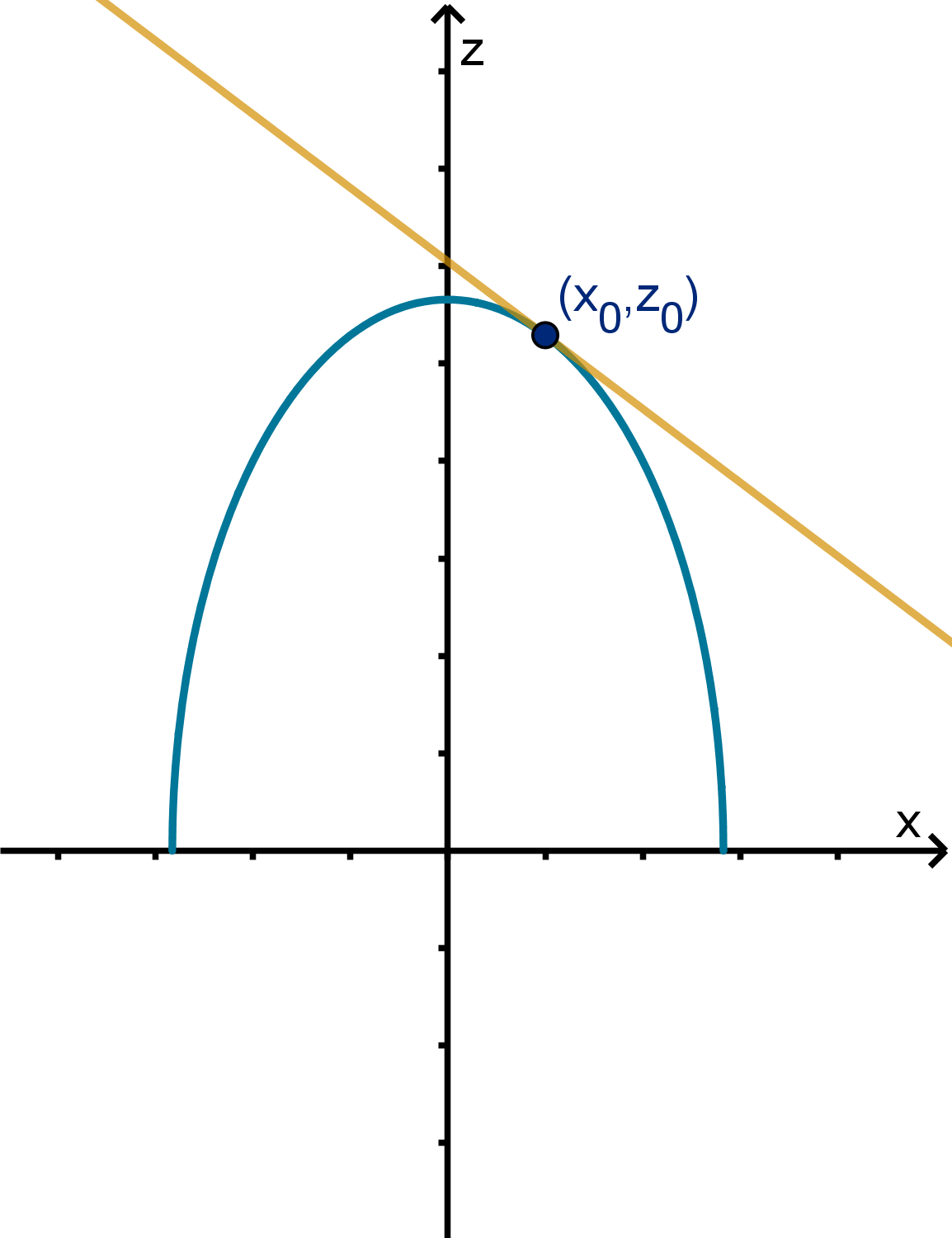
Figure: The tangent line to z = f(x, y) in the x direction
Definition
Let f(x, y) be a function and u be a unit vector in R
2
. The directional derivative, denoted D
u
f,
is the instantaneous rate of change of f as we move in the u direction. This is also the slope of the
tangent line to y = f(x, y) in the direction of u.
342
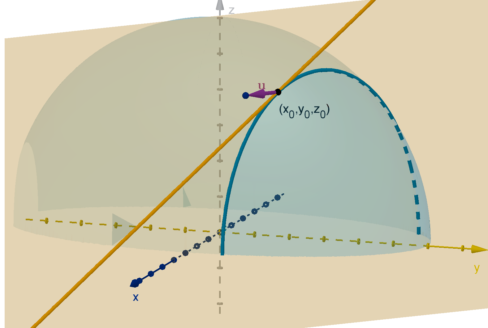
Figure: The tangent line to f(x, y) in the direction of u
Recall that we compute D
x
f by comparing the values of f at (x, y) to the value at (x + h, y), a
displacement of h in the x-direction.
D
x
f(x, y) = lim
h→0
f(x + h, y) − f (x, y)
h
To compute D
u
f for u = a
i+b
j, we compare the value of f at (x, y) to the value at (x+ta, y +tb),
a displacement of t in the u-direction.
Limit Formula
D
u
f(x, y) = lim
t→0
f(x + ta, y + tb) − f(x, y)
t
Questions:
1 What direction produces the greatest directional derivative? The smallest?
2 How are these directions related to the geometry (specifically the level curves) of the graph?
3 How these directions related to the partial derivatives?
We can explore these questions with an applet in the Other Cross Sections activity.
343
Question 5.4.1
How Do We Compute Rates of Change in Another Direction?
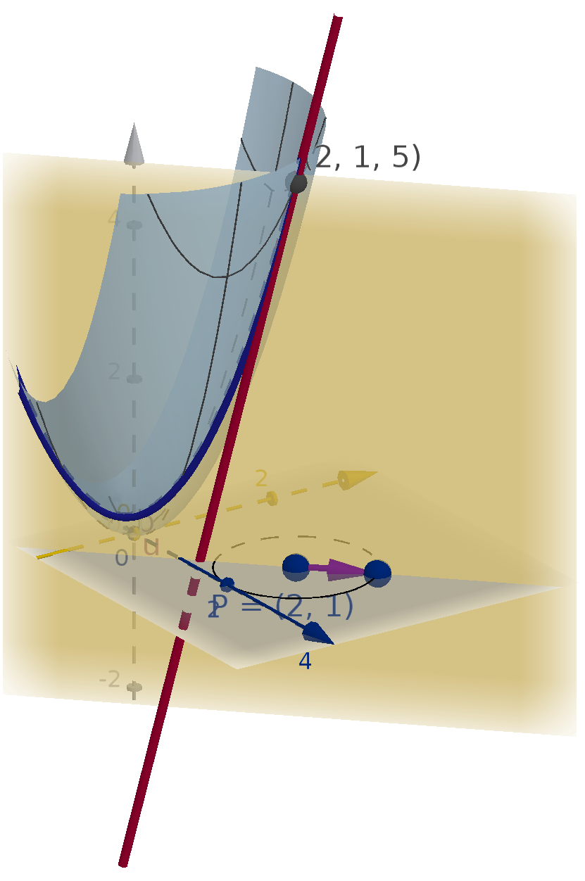
Figure: A cross section of z = f(x, y) and a tangent line in the direction of u
Question 5.4.2
What Is the Gradient Vector?
The relationship between the direction of maximum increase and the partial derivatives suggest that
we could treat the partial derivatives like components of a vector.
Definition
The gradient vector of f at (x, y) is
∇f(x, y) = ⟨f
x
(x, y), f
y
(x, y)⟩
Remarks:
1 The gradient vector is a function of (x, y). Different points have different gradients.
2 u
max
, which maximizes D
u
f, points in the same direction as ∇f .
3 u
0
, which is tangent to the level curves, is orthogonal to ∇f.
344
Remark
Students often wonder: what is the geometric intuition behind the gradient vector and its properties?
The answer is often disappointing, but important. The gradient vector does not have a geometric
motivation. We artificially created the gradient vector because it has convenient algebraic properties. If
that were the end of the story, we wouldn’t bother learning about it. However, the gradient turns out
to be so useful that we will study it intensely, despite its uncompelling origins.
Question 5.4.3
How Do We Compute a Directional Derivative?
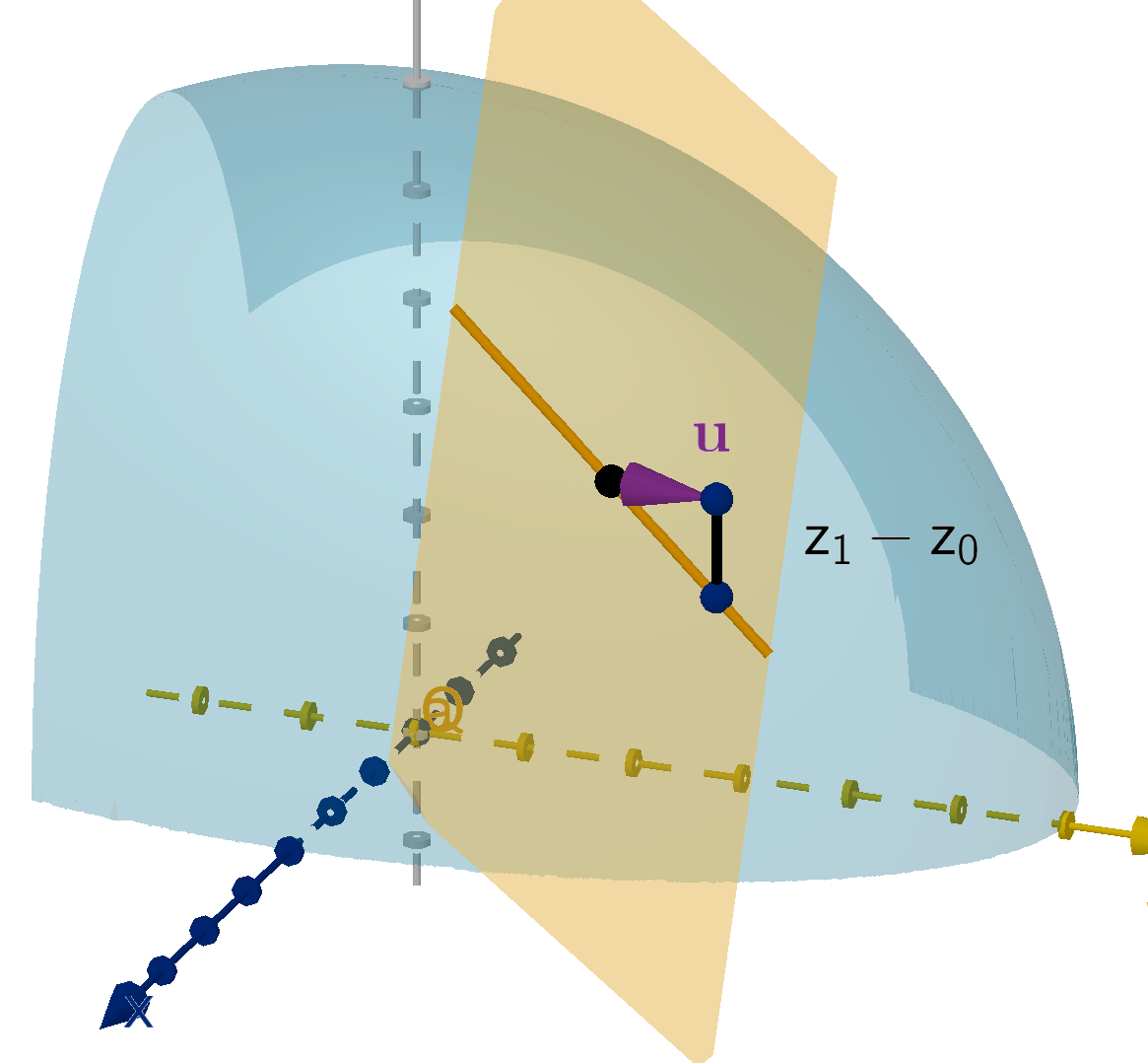
There are several ways to derive a formula for the directional derivative. One approach is to apply
algebra and limit laws to the limit definition. A more geometric method is to exploit our previous work
with the tangent plane. The directional derivative is the slope of a tangent line. The tangent lines live
in the tangent plane. We can compute their slope by rise over run.
Let u be a unit vector from (x
0
, y
0
) to (x
1
, y
1
). Let the associated z values in the tangent plane be
z
0
and z
1
respectively.
D
u
f(x
0
, y
0
) =
rise
run
=
z
1
− z
0
|u|
=f
x
(x
0
, y
0
)(x
1
− x
0
) + f
y
(x
0
, y
0
)(y
1
− y
0
)
=∇f(x
0
, y
0
) · u.
Functions of More Variables
We can also define directional derivatives of higher variable functions with analogous results.
f(x
1
, . . . , x
n
) is a differentiable function.
u is a unit vector in R
n
.
D
u
f denotes the directional derivative in the direction of u.
∇f = ⟨f
x
1
, . . . , f
x
n
⟩ is an n-dimensional vector function on R
n
.
D
u
f = ∇f · u
345
Synthesis 5.4.4
Directional Derivative and the Cosine Formula
Now that we have a formula for directional derivatives, we can verify our observations from earlier.
Suppose f(x, y) is a differentiable function and we can choose any unit vector u.
a
Write D
u
f(x, y) in terms of the length of a vector and an angle.
b
In what direction u will f increase fastest?
c
What will be the value of D
u
f(x, y) in that direction?
d
In what direction u will D
u
f(x, y) = 0?
Solution
a
Since the directional derivative is a dot product, we can apply our formula that relates the dot
product to the lengths of the vectors and the angle between them.
D
u
f(x, y) = ∇f(x, y) ·u dot product formula
= |∇f(x, y)||u|cos θ cosine formula
= |∇f(x, y)|cos θ u is a unit vector
b
Given a particular (x, y), |∇f(x, y)|cos θ is largest when θ = 0 This means that D
u
f(x, y) is
maximized when u is in the direction of ∇f(x, y). The formula for a unit vector in the direction
of the gradient is
u =
1
|∇f(x, y)|
∇f(x, y)
c
In this direction, cos θ = 1 so D
u
f(x, y) = |∇f(x, y)|.
d
We can solve for θ
D
u
f(x, y) = 0
|∇f(x, y)|cos θ = 0by part (a)
cos θ = 0 as long as ∇f (x, y) =
0
θ =
π
2
We conclude that u must be orthogonal to ∇f(x, y).
346
Figure: The angle between the gradient of f and a unit vector
Main Ideas
The cosine formula for the dot product lets us relate the directional derivative to an angle.
f increases fastest in the direction of ∇f(x, y).
D
u
f(x, y) = 0 when ∇f(x, y) and u are orthogonal.
Example 5.4.5
A Directional Derivative
Let f(x, y) =
p
9 − x
2
− y
2
and let u = ⟨0.6, −0.8⟩.
a
What are the level curves of f?
b
What direction does ∇f (1, 2) point?
c
Without calculating, is D
u
f(1, 2) positive or negative?
d
Calculate ∇f(1, 2) and D
u
f(1, 2).
347
Example 5.4.5
A Directional Derivative
Solution
a
The level curves have the equations
p
9 − x
2
− y
2
= c. These solve to x
2
+ y
2
= 9 − c
2
. As
c increases from 0 to 3 these are circles starting at radius 3 and shrinking to the origin. For c
outside this range, the level curve has no points.
b
∇f points in the direction of increase and normal to the level curves. Since higher level curves
are smaller circles, closer to the origin, ∇f (1, 2) points toward the origin.
c
D
u
f(1, 2) = ∇f(1, 2) ·u. Since u appears to make an acute angle with ∇f(1, 2), we expect this
dot product to be positive.
d
First we need to compute ∇f (1, 2).
∇f(x, y) = ⟨f
x
(x, y), f
y
(x, y)⟩
=
*
1
2
p
9 − x
2
− y
2
(−2x),
1
2
p
9 − x
2
− y
2
(−2y)
+
(chain rule)
∇f(1, 2) =
1
2
√
9 − 1
2
− 2
2
(−2)(1),
1
2
√
9 − 1
2
− 2
2
(−2)(2)
=
−
1
2
, −1
Now we use the dot product formula to compute D
u
f(1, 2).
D
u
f(1, 2) = ∇f(1, 2) · u
=
−
1
2
, −1
· ⟨0.6, −0.8⟩
348
= −0.3 + 0.8
= 0.5
This confirms our intuition that D
u
f(1, 2) is positive.
Example 5.4.6
Drawing the Gradient
Let h(x, y) give the altitude at longitude x and latitude y. Assuming h is differentiable, draw the
direction of ∇h(x, y) at each of the points labeled below. Which gradient is the longest?
A
B
C
Figure: A topographical map
Solution
The gradient vector at each point is normal to the level curves, pointing uphill. The hill is steepest at
B, because the level curves are closer together. This tells us that the partial derivatives are larger. Thus
∇h(B) is longer than ∇h(A) and ∇h(C).
A
B
C
349
Application 5.4.7
Edge Detection
Representing an image by defining a brightness (or color) function on the pixels is simple enough,
but can a computer be taught to make sense of what it sees? Image recognition is an exciting field that
promises to automate and improve tasks from medical diagnosis to driving a vehicle.
The problem is daunting. What algorithm can possibly take a set of pixels and locate a tumor or a
pedestrian? The first step is to identify the objects in the image. The first step of object identification is
edge detection, determining where one object ends and another begins. We can do this by approximating
the partial derivatives at each pixel. We compare each pixel to nearby pixels and compute rise over run
(how these are chosen and averaged can significantly affect the accuracy of the algorithm).
The length of the gradient of a brightness function detects the edges in a picture, where the brightness
is changing quickly.
∂B
∂x
(336, 785) ≈
185−187
1
∂B
∂y
(336, 785) ≈
179−187
1
∇B(336, 785) ≈ (−2, −8)
∂B
∂x
(340, 784) ≈
97−139
1
∂B
∂y
(340, 784) ≈
72−139
1
∇B(340, 784) ≈ (−42, −67)
∇B
∇B
Figure: A long gradient vector indicates a swift change in brightness. Its direction suggests the shape
of the edges.
Notice that the gradient is long near the edge of the iris in Mona Lisa’s eye. It is much shorter at a
point in the white of her eye. Moreover, the gradient at the edge of the iris is approximately normal to
the edge of her iris, because gradients are normal to level curves. This information can be used by an
algorithm to detect not only the location of the edges, but also their direction.
Application 5.4.8
Tangent Planes to a Level Surface
Use a gradient vector to find the equation of the tangent plane to the graph x
2
+ y
2
+ z
2
= 14 at
the point (2, 1, −3).
There are two solutions worth comparing here.
350
Solution 1
We can write z as a function of x and y and apply the tangent plane formula.
x
2
+ y
2
+ z
2
= 14
z
2
= 14 − x
2
− y
2
z = −
p
14 − x
2
− y
2
(z = −3 is on the negative branch of the function)
f
x
(x, y) = −
1
2
p
14 − x
2
− y
2
(−2x) f
x
(2, 1) =
2
3
f
y
(x, y) = −
1
2
p
14 − x
2
− y
2
(−2y) f
y
(2, 1) =
1
3
Equation: z + 3 =
2
3
(x − 2) +
1
3
(y − 1)
Solution 2
Define F (x, y, z) = x
2
+ y
2
+ z
2
. The graph x
2
+ y
2
+ z
2
= 14 is a level surface of F . ∇F (2, 1, −3)
is normal to the level surface, meaning it is also a normal vector for the tangent plane.
∇F (x, y, z) = ⟨2x, 2y, 2z⟩
∇F (2, 1, −3) = ⟨4, 2, −6⟩
We now have a normal vector n = ∇F (2, 1, −3). Our known point is (x
0
, y
0
, z
0
) = (2, 1, −3). The
normal equation of the plane is
4(x − 2) + 2(y − 1) − 6(z + 3) = 0.
Solution 2 requires more conceptual reasoning, but is computationally much easier. In fact, in
some cases we cannot use Solution 1 at all because we do not know how to solve for z. Once we are
comfortable with the concepts involved, the second method is generally superior for graphs of implicit
equations.
351
Application 5.4.8
Tangent Planes to a Level Surface
Main Idea
The graph of an implicit equation can be written as a level set of a function. The gradient of that
function is a normal vector to the level set and also to its tangent line/plane/hyperplane.
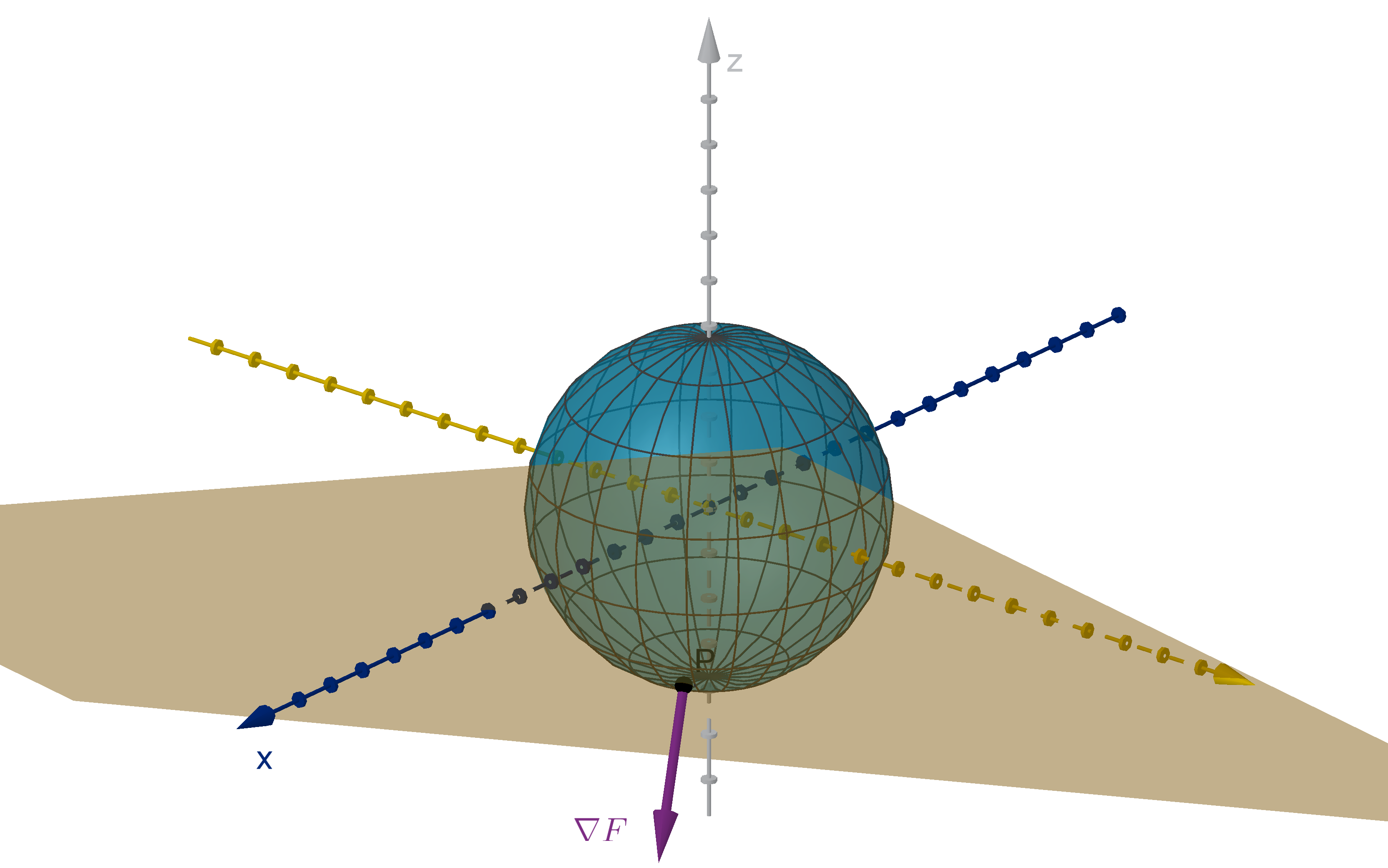
Figure: The level surface x
2
+ y
2
+ z
2
= 14, its tangent plane and ∇F .
Section 5.4
Exercises
Summary Questions
Q1
What does the direction of the gradient vector tell you?
Q2
What does the directional derivative mean geometrically?
Q3
How do you compute a directional derivative?
Q4
How is the gradient vector related to a level set?
352
5.4.1
Q5
Suppose that f(3, 7) = 12 and f (7, 4) = 10.
a
What is the distance from (3, 7) to (7, 4)?
b
Approximate the rate of change of f at (3, 7) travelling toward (7, 4)
Q6
Suppose g(0, 2) = 15 and g(4, 1) = 17.
a
What is the distance from (0, 2) to (4, 1)?
b
Approximate the rate of change of g at (0, 2) travelling toward (4, 1).
c
If you wanted to express the previous rate of change as an approximation of D
u
g(0, 2), what
would the unit vector u be?
5.4.2
Q7
If f(x, y) = x
2
sin(xe
y
), what is ∇f (x, y)?
Q8
If g(x, y) =
p
6x
2
+ 5y
4
, what is ∇g(x, y)?
Q9
If ∇f(x
0
, y
0
) is orthogonal to ∇g(x
0
, y
0
), what can we say about the level curves of f and g?
Be specific.
Q10
Harriet says “The gradient vector of f is tangent to the graph of z = f(x, y).”
“No,” says Marcus, “it is normal to the graph of z = f(x, y).” Who is correct?
353
Section 5.4
Exercises
5.4.3
Q11
Consider our computation of the directional derivative as a dot product.
a
Where did we use the fact that u is a unit vector?
b
If u were not a unit vector, then ∇f ·u would no longer represent rise over run. What would
it represent instead?
Q12
Suppose the linearization of f (x, y) at (−3, 9) has the equation
L(x, y) = 4 + 2(x + 3) −
1
3
(y − 9).
What is the slope of L from (−3, 9) to (5, 3)?
5.4.4
Q13
Given a function f(x, y) and a point (x, y), in what direction u is f decreasing fastest? Compute
an expression for u.
Q14
If D
u
f(x, y) < 0, what can you say about the directions of ∇f(x, y) and u?
Q15
If f
x
(3, 5) = f
y
(3, 5) in what direction(s) from (3, 5) could f increase most quickly?
Q16
Explain why it makes sense that if D
u
f(a, b, c) = 0, then u is tangent to the level surface of f
through (a, b, c).
Q17
If f(x, y, z) = 3xy + z
2
, find the unit vector u that maximizes D
u
f(2, 1, −4). What is the value
of D
u
f(2, 1, −4) for this u?
Q18
Let f(x, y) = 2x
2
y − 10x − y
2
.
a
What unit vector u maximizes the quantity D
u
f(−1, 3)?
b
Compute D
u
f(−1, 3) for the u you found in part
a
.
354
5.4.5
Q19
If u =
2
3
, −
1
3
, −
2
3
and f(x, y, z) = xe
yz
, compute D
u
f(3, 0, 4).
Q20
If u =
3
7
,
6
7
, −
2
7
and f(x, y, z) = xy + yz + zx, compute D
u
f(7, −7, 14).
Q21
If u is a unit vector in the direction of ⟨2, 3⟩ and f(x, y) = x
2
+ 3xy + 2, calculate D
u
f(−1, 4).
Q22
Compute the directional derivative of g(x, y) = e
x
2
−y
at (3, 7) in the direction of ⟨−12, 5⟩.
5.4.6
Q23
In this diagram, we have several level sets of f(x, y).
a
Which way does ∇f (−4, 1.25) point?
b
Mark all the points (x, y) that satisfy
f(x, y) = 30
∇f(x, y) points in the positive y-direction
Q24
Some level curves of f are drawn below. Indicate the direction of the gradient of f at each
labelled point.
355
Section 5.4
Exercises
5.4.7
Q25
If ∇B(x
0
, y
0
) = ⟨13, −17⟩, would you expect the pixels above (x
0
, y
0
) to be brighter or dimmer
than (x
0
, y
0
)? Explain.
Q26
The brightness function on the Mona Lisa image ranges from 0 to 255. If we use adjacent points
to apporixmate the gradient as in the example, what is the longest gradient vector we could
theoretically produce?
5.4.8
Q27
Calculate a normal equation of a tangent line to x
3
+ 8y
3
− 12xy = 0 at (3, 1.5).
Q28
Let P be a point on the circle x
2
+ y
2
= r
2
. Show that the position vector of P is normal to the
circle at P .
Q29
Produce an equation of the tangent plane to z
3
− xz
2
− yx
2
= 24 at (4, −2, 2).
Q30
Give an equation of the tangent plane to the graph z
2
x + 2yz − x
2
y
2
= 59 at (3, 2, 5).
356
Synthesis and Extension
Q31
Suppose f(x, y) is a differentiable function, and we know that for u = ⟨−0.6, 0.8⟩, D
u
f(5, −1) =
4 and for v = ⟨0, −1⟩ we know that D
v
f(5, −1) = −2. What is ∇f (5, −1)?
Q32
Suppose the point P = (x
0
, y
0
, z
0
) lies on the graph z = f(x, y).
a
Give the formula for tangent plane to this graph at P .
b
z = f (x, y) is a level surface of F (x, y, z) = f (x, y) −z. Use the gradient of F to write the
equation of the tangent plane to F (x, y, z) = 0 at P .
c
Are these equations equivalent? Justify your answer with algebra.
Q33
How could you use the gradient of f to rewrite the formula for the linearization L(x, y) of f(x, y)
at (x
0
, y
0
)?
Q34
Suppose f(x, y) is a differentiable function and ∇f (a, b) is not the zero vector. How many unit
vectors u exist such that D
u
f(a, b) = 0. How are they related geometrically?
Q35
Suppose f(x, y, z) is a differentiable function and ∇f(a, b, c) is not the zero vector. How many
unit vectors u exist such that D
u
f(a, b, c) = 0. How are they related geometrically?
Q36
Suppose that f(x, y, z) is a differentiable function, and f(3, 5, −2) = 13. Suppose further that
the vectors ⟨3, 1, 0⟩ and ⟨0, 2, 5⟩ both lie in the tangent plane to the surface f (x, y, z) = 13 at
(3, 5, −2). If the maximum value of D
u
f(3, 5, −2) is 20, find all possible values of ∇f(3, 5, −2).
Q37
Consider the function h(x, y) = x
2
+ 2x + 4y
3/2
a
Compute all possible unit vectors u such that D
u
h(2, 3) = 6
b
What angle do these vectors u make with the tangent line to the level curve h(x, y) =
8 + 12
√
3 at (2, 3).
Q38
Let f(x, y) = x
4
y + 3x − y
3
.
a
Give an equation of the level curve of f through the point (−1, 2).
b
Give an equation of the tangent line to the level curve of f at (−1, 2). Write your equation
in normal form.
357
Section 5.4
Exercises
c
Give an expression for the linearization of f at (−1, 2).
358
Section 5.5
The Chain Rule
Goals:
1 Use the chain rule to compute derivatives of compositions of functions.
2 Perform implicit differentiation using the chain rule.
Motivational Example
Suppose Jinteki Corporation makes widgets which is sells for $100 each. It commands a small enough
portion of the market that its production level does not affect the demand (price) for its products. If
W is the number of widgets produced and C is their operating cost, Jinteki’s profit is modeled by
P = 100W − C
The partial derivative
∂P
∂W
= 100 does not correctly calculate the effect of increasing production on
profit. How can we calculate this correctly?
Question 5.5.1
How Can We Visualize a Composition with a Multivariable Function?
You may recall parametric equations from high school algebra. A parametric equation actually
consists of two or more equations. Each expresses a variable in our coordinate system in terms of a
parameter t.
We can visualize a parametric equation as particle traveling through space.
The variable t represents time.
x(t) and y(t) represent the coordinates of the position at time t.
The vector ⟨x
′
(t), y
′
(t)⟩ represents velocity. It points in the direction of travel.
Figure: A particle whose position is defined by x(t) and y(t), the path it follows and its velocity vector
359
Question 5.5.1
How Can We Visualize a Composition with a Multivariable Function?
Given a function f(x, y) where x = x(t) and y = y(t), we can ask how f changes as t changes.
We can visualize this change by drawing the graph z = f(x, y) over the path given by the parametric
equations x(t) and y(t).
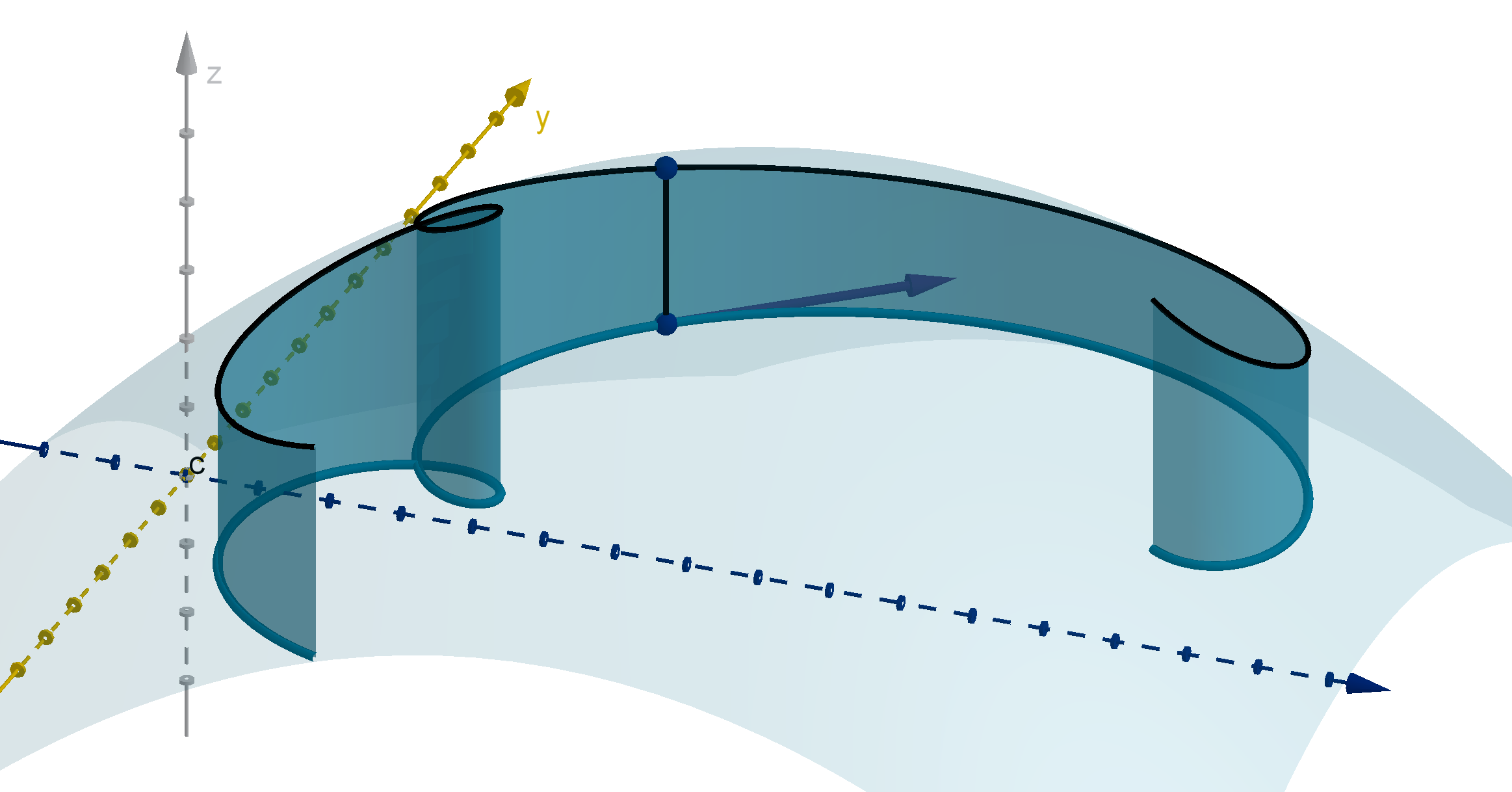
Figure: The composition f (x(t), y(t)), represented by the height of z = f(x, y) over the path
(x(t), y(t))
Question 5.5.2
How Do We Compute the Derivative of a Composition of Functions?
Theorem [The Chain Rule]
Consider a differentiable function f(x, y). If we define x = x(t) and y = y(t), both differential functions,
we have
df
dt
=
∂f
∂x
dx
dt
+
∂f
∂y
dy
dt
or
df
dt
= ∇f(x, y) · ⟨x
′
(t), y
′
(t)⟩
360
Remarks
f(x(t), y(t)) is a function (only) of t. Because of this,
df
dt
is an ordinary derivative, not a partial
derivative.
df
dt
is not the slope of the composition graph.
slope =
rise in z
run in xy-plane
df
dt
=
rise in z
change in t
The chain rule is easy to remember because of its similarity to the differential:
dz =
∂z
∂x
dx +
∂z
∂y
dy.
The proof is more complicated than just sticking a dt under each term.
Example 5.5.3
Using the Chain Rule
If P = R − C and we have R = 100w and C = 3000 + 70w − 0.1w
2
, calculate
dP
dw
.
Solution
The chain rule says
dP
dw
=
∂P
∂R
dR
dw
+
∂P
∂C
dC
dw
We compute the required partial derivatives:
∂P
∂R
= 1
∂P
∂C
= −1
dR
dw
= 100
dC
dw
= 70 − 0.2w
We plug these into the formula to get
dP
dw
= (1)(100) + (−1)(70 − 0.2w)
= 30 + 0.2w
361
Example 5.5.3
Using the Chain Rule
Remark
Notice we don’t need the chain rule when we have expressions for each function. We can write the
composition ourselves and take an ordinary derivative. In this example we could just differentiate
P = 100w − (3000 + 70w − 0.1w
2
).
Question 5.5.4
What If We Have More Variables?
The chain rule works just as well if x and y are functions of more than one variable. In this case it
computes partial derivatives.
Theorem
If f(x, y), x(s, t) and y(s, t), are all differentiable, then
∂f
∂s
=
∂z
∂x
∂x
∂s
+
∂z
∂y
∂y
∂s
or
∂f
∂s
= ∇f(x, y) ·
∂x
∂s
,
∂y
∂s
We can also modify it for functions of more than two variables.
Theorem
Given f(x, y, z), x(t), y(t) and z(t), all differentiable, we have
df
dt
=
∂f
∂x
dx
dt
+
∂f
∂y
dy
dt
+
∂f
∂z
dz
dt
or
df
dt
= ∇f(x, y, z) · ⟨x
′
(t), y
′
(t), z
′
(t)⟩
362
Example 5.5.5
A Composition with More Variables
Recall that for an ideal gas P (n, T, V ) =
nRT
V
. R is a constant. n is the number of molecules of
gas. T is the temperature in Celsius. V is the volume in meters. Suppose we want to understand the
rate at which the pressure changes as an air-tight glass container of gas is heated.
a
Apply the chain rule to get an expression for
dP
dT
.
b
What is
dn
dT
?
c
What is
dT
dT
?
d
Suppose that
dV
dT
= (5.9 × 10
−6
)V . Calculate and simplify the expression you got for
dP
dT
.
Solution
a
dP
dT
=
∂P
∂T
dT
dT
+
∂P
∂n
dn
dT
+
∂P
∂V
dV
dT
b
The container is sealed so no molecules are getting in or out.
dn
dT
= 0.
c
If we write T as a function of T , we get T = T .
dT
dT
= 1.
d
We’ll compute the partial derivatives and then plug them into our chain rule expression.
∂P
∂T
=
nR
V
∂P
∂V
= −
nRT
V
2
dP
dT
=
nR
V
(1) + 0 −
nRT
V
2
(5.9)(10
−6
)V
=
nR(1 − 0.0000059T )
V
363
Example 5.5.6
A Composition with Limited Information
Suppose g(p, q, r) = re
p
2
q
. Given that p, q, r are all differentiable functions of x with the values in
the following table, compute
dg
dx
when x = 2.
x 0 1 2 3
p(x) 3 1 5 10
p
′
(x) −3 2 3 4
q(x) 6 2 −2 3
q
′
(x) −1 −5 2 3
r(x) 10 11 7 3
r
′
(x) 1 0 −1 −3
Solution
The chain rule says
dg
dx
=
∂g
∂p
dp
dx
+
∂g
∂q
dq
dx
+
∂g
∂r
dr
dx
We require the partial derivatives of g
∂g
∂p
= 2pqre
p
2
q
∂g
∂q
= p
2
re
p
2
q
∂g
∂r
= e
p
2
q
Now we plug in the partial derivatives, along with the derivatives of p, q and r from the table.
dg
dx
= 2pqre
p
2
q
(3) + p
2
re
p
2
q
(2) + e
p
2
q
(−1)
This is correct, but not sufficiently simplified. We have left p’s, q’s and r’s in the expression, but the
table tells us what value these have when x = 2. We can make these subsitutions:
dg
dx
= 2(5)(−2)(7)e
(5)
2
(−2)
(3) + (5)
2
(7)e
(5)
2
(−2)
(2) + e
(5)
2
(−2)
(−1)
= −420e
−50
+ 350e
−50
− e
−50
= −71e
−50
364
Application 5.5.7
Implicit Differentiation
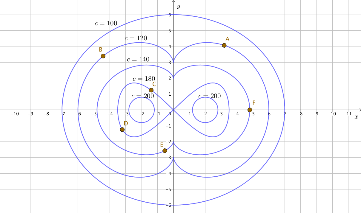
Recall that an implicit equation on n variables is a level curve of a n-variable function. Consider the
graph x
3
+ y
2
− 4xy = 0. How can we use this to calculate
dy
dx
at the point (3, 3)?
Solution
First, note that (3, 3) does lie on the graph. When we plug x = 3 and y = 3 into our equation, we get
27 + 9 − 36 = 0, which is true. Now suppose that for every x near 3, we can define y(x) to be the y
coordinate on the graph x
3
+ y
2
− 4xy = 0.
Define F (x, y) = x
3
+ y
2
−4xy. The points (x, y(x)) lie on the graph F (x, y) = 0. We can use this
equation to obtain an expression for
dy
dx
. When we differentiate F (x, y(x)), both components change as
x changes, so we cannot use a partial derivative. We need the chain rule.
F (x, y(x)) = 0
d
dx
F (x, y(x)) =
d
dx
0 differentiate both sides
∂F
∂x
dx
dx
+
∂F
∂y
dy
dx
= 0 apply chain rule
∂F
∂x
+
∂F
∂y
dy
dx
= 0
dx
dx
= 1
∂F
∂y
dy
dx
= −
∂F
∂x
solve for
dy
dx
dy
dx
= −
∂F
∂x
∂F
∂y
We compute the partial derivatives at (3, 3), then plug them into the formula we derived.
F
x
(x, y) = 3x
2
− 4y F
x
(3, 3) = 15
F
y
(x, y) = 2y − 4x F
y
(3, 3) = −6
dy
dx
= −
15
−6
=
5
2
Figure: The graph of F (x, y) = x
3
+ y
2
− 4xy = 0, its tangent line at (3, 3), and the gradient of F
365
Application 5.5.7
Implicit Differentiation
Main Ideas
dy
dx
is the slope of the tangent line to F (x, y) = c.
The chain rule allows us to derive
dy
dx
= −
F
x
F
y
−
F
x
F
y
is the negative reciprocal of
F
y
F
x
, which is the slope of ∇F .
In order to solve for
dy
dx
we had to assume that y was a differentiable function of x. How do we
know that’s even true? There is an advanced and powerful theorem that tells us when we can write one
variable in an implicit equation as a function of the others. Here is the two-variable version.
Theorem [The Implicit Function Theorem]
Suppose we have a point (x
0
, y
0
) on the graph of F (x, y) = c. Suppose that
1 The partial derivatives of F exist and are continuous at (x
0
, y
0
)
2 F
y
(x
0
, y
0
) = 0
Then there is a function y = f(x) that agrees with the graph of F (x, y) = c in some neighborhood
around (x
0
, y
0
). Furthermore
1 f is continuous
2 f is differentiable
3 f
′
(x
0
) = −
F
x
(x
0
, y
0
)
F
y
(x
0
, y
0
)
In the case of our example, the partial derivatives in question are polynomials. As long as F
y
(x
0
, y
0
) =
0, we are guaranteed that our graph has a tangent line at (x
0
, y
0
), and its slope is −
F
x
(x
0
, y
0
)
F
y
(x
0
, y
0
)
.
Application 5.5.8
Indirect Profit Functions
Suppose a firm chooses how much quantity q to produce, but their profit Π(q, α) depends on some
parameter α outside their control (maybe a tax or a measure of regulatory burden). The firm, once
it knows the value of α, will choose the q that maximizes profit. How will their profit change as α
changes?
366
Solution
The change in the firms profit is
dΠ
dα
. Since q is also a function of α we will need the chain rule.
dΠ
dα
=
∂Π
∂q
dq
dα
+
∂Π
∂α
dα
dα
We can substitute
dα
dα
= 1. We can also argue that
∂Π
∂q
= 0. Why? Because q is the choice that
maximizes profit, and maximums occur at critical points. If
∂Π
∂q
> 0 then the firm could increase q to
increase profit (without changing α, which it has no control over). Similarly, If
∂Π
∂q
< 0 then reducing
production would increase profit.
Performing these substitutions gives:
dΠ
dα
=
∂Π
∂α
This suggests that in this case, the total derivative is equal to the partial derivative.
We can verify this equality graphically as well. Pick a particular α
0
and let q
0
= q(α
0
). Notice:
The graph π(q
0
, α) is never above π(q(α), α) for any α, since q(α) is the optimal choice of q.
The graphs π(q
0
, α) and π(q(α), α) meet at α
0
, since q
0
= q(α
0
).
If two graphs meet but one stays below the other, they are tangent. They have the same tangent
line and thus the same derivative.
Figure: Two graphs of z = Π(q, α), one where q changes to be the optimal choice for each α and one
where q is fixed at q
0
, the optimal choice for α
0
367
Application 5.5.8
Indirect Profit Functions
Remark
If we had an expression for q(α) and an expression for Π, we could substitute and use ordinary differen-
tiation. Since we did not, we needed the chain rule. Even with such an expression, to find
dΠ
dα
directly
we would need to
1 Solve for q as a function of α
2 Substitute q(α) into Π(q, α)
3 Differentiate the result
Taking a partial derivative is less work. Our result (which economists call the envelope theorem) is
both a useful abstraction and a computational shortcut.
Section 5.5
Exercises
Summary Questions
Q1
How can we visualize f (x, y), when x and y are functions of t?
Q2
Explain why
df
dt
cannot be interpreted as a slope of f over the xy-plane.
Q3
What is the difference between
dz
dx
and
∂z
∂x
? How is the first one computed?
Q4
How do you use the chain rule to differentiate implicit functions?
5.5.1
Q5
Plug in a few different t values and plot the corresponding points of
x(t) = 3 + 5t
y(t) = −2 + 4t
What is the resulting curve? What is the significance of the t coefficients?
368
Q6
Consider the curve defined by
x(t) = t
y(t) = e
t
a
Plot a few points on the curve by plugging in different values of t.
b
In general, what curve does
x(t) = t
y(t) = f(t)
seem to produce?
Q7
A particle is travelling according to the parametric equations
x(t) = 2 cos t
y(t) = 3 sin t
What is the speed (magnitude of velocity) at t =
π
3
?
Q8
Produce a tangent vector to the curve defined by
x(t) = t
3
y(t) = t
2
at the point (−27, 9).
Q9
Is the graph of
x(t) = t
2
y(t) = sin(t)
the graph of a function? How can you tell without graphing it?
Q10
How are the graphs of the following two parametric equations related? Can you generalize your
answer to similar pairs of parametric equations?
x(t) = cos t x(t) = cos(t
3
)
y(t) = ln t y(t) = ln(t
3
)
369
Section 5.5
Exercises
5.5.2
Q11
Let f(x, y) be a funtion. Under what conditions is
df
dt
equal to the directional derivative of f in
the direction of the tangent vector ⟨x
′
(t), y
′
(t)⟩?
Q12
Liam says “If f is a function of x and y and x and y are increasing, then f is increasing.” We
all know Liam is incorrect. How could we use the chain rule to refute him?
5.5.3
Q13
The angular speed of an object is given by ω =
v
r
where r is the distance from the center of
rotation and v is the linear speed. Suppose an object is orbiting earth at a radius of 8400000m
and a speed of 6900m/s. If the radius is increasing at a rate of 100m/s and the linear speed is
decreasing by 60m/s
2
, how quickly is the angular speed changing?
Q14
Let x = t
2
and y = sin t. Let f (x, y) = xy.
a
Compute
df
dt
using the multivariable chain rule.
b
Compute
df
dt
by substituting and using single-variable differentiation.
c
What earlier rule of differentiation can we recover by applying the chain rule to f(x, y) = xy?
5.5.4
Q15
Suppose h(x
1
, x
2
, x
3
, x
4
) is a four-variable function and each x
i
(x, t) is a function of parameters
s and t. How would the multivariable chain rule compute
∂h
∂t
?
Q16
Suppose k(x) is a function and x(r, s, t) is a function of paramters r, s, and t. How does the
multivariable chain rule say we should compute
∂k
∂r
?
370
5.5.5
Q17
Agular momemtum is given by L = rmv where r is the radius of roatation, m is the mass of the
object, and v is its linear speed. At a certain time t
0
, r is 42 million meters and increasing at
80, 000 meters per second, m is 6000kg and not changing, and v is 3100m/s and increasing at
20m/s
2
. How quickly is angular momentum increasing?
Q18
Let f(x, y) = x
2
−y
2
. If x(r, θ) = r cos θ and y(r, θ) = r sin θ, compute
∂f
∂θ
at (r, θ) =
4,
π
6
.
5.5.6
Q19
Suppose x(t) and y(t) are differentiable functions of t such that
x(2) = 3 x
′
(2) = 2 y(2) = −5 y
′
(2) = 10
If f(x, y) = ye
(x
2
y)
, show how to compute
df
dt
at t = 2.
Q20
Suppose that x and y are functions of t such that when t = 2:
x = 3 y = 1
dx
dt
= 5
dy
dt
= 2
If g(x, y) = 3xy
2
− x
2
+ 2y, compute
dg
dt
t=2
.
5.5.7
Q21
Compute
dy
dx
at (4, 2), if x and y satisfy y
3
− xy + x
2
− 4 = 0
Q22
Compute
dy
dx
at (3, 0), if x and y satisfy xe
xy
= 3
Q23
What is the slope of the tangent line to x − y
2
= 9 at (18, −3)?
Q24
Compute the slope of the tangent line to x
3
= y
2
at (4, −8).
371
Section 5.5
Exercises
Q25
Angular momentum is given by L = rmv. One law of physics states that angular momentum of
an object is conversed (unchanged) unless the a force (besides gravity) acts to speed up or slow
down the object. Use the chain rule to derive an expression for
dv
dr
, the amount of linear speed
an object gains or loses per unit that its radius of rotation increases. What do you notice about
the role of mass in your answer?
Q26
Another principle in physics is the conservation of energy. Kenetic energy is given by E =
1
2
mv
2
,
where m is the mass and v is the linear speed of the object. Suppose that we have a rock
drifiting through space. Suppose it impacts stationary rocks and the combined mass sticks
together (without releasing any energy as heat, light or sound). Thus the mass of the total
travelling object increases, while the total energy stays the same. Derive an expression for how
speed changes per unit of increase in mass.
5.5.8
Q27
Suppose that x is a function of t and that when t = 9, we have x = 7 and
dx
dt
= −3. Define
f(x, t) =
√
x + t.
a
Compute the partial derivate
∂f
∂t
(7, 9).
b
Compute the total derivative
df
dt
(7, 9).
c
In a few sentences, explain what these two quantities compute and why they are different
from each other.
Q28
A firm with a monopoly produces gets to set the price of its products and decide how much to
produce. There is a demand function p such that if the firm produces q units, it must set its
price at p(q) to get consumer to buy all of its production. Each unit costs c to produce. The
profit function of the firm is
π(q, c) = p(q)q − cq
We can assume that once the firm has worked out what c is, it chooses the q to maximize profit.
How much will the firm’s actual profit change per unit of increase in c?
372
Synthesis and Extension
Q29
Find the slope of the tangent line to x
2
+ 2x −y
2
= 8 at (5, −3) using each of the following two
methods.
a
Using a gradient vector to write the normal equation of the line and solving for the slope.
b
Using implicit differentiation.
Q30
Suppose the position of a particle at time t is given by
x(t) = t
2
y(t) = 3 − t
z(t) =
√
t
At t = 4, how quickly is particle travelling away from the plane x + 2y − 2z = 10?
Q31
Here is a diagram of the level curves of h(x, y) for certain values of c.
a
Is h
y
(2, 1) positive or negative? Explain in a sentence or two.
b
Add a vector to the diagram that indicates the direction of greatest increase of h at (−2, 0).
c
Suppose x = 4 −5t and y = 3t
2
. Determine, with the aid of a relevant calculation, whether
dh
dt
is positive or negative at t = 1.
Q32
Let f(x, y) = x
5
+ 20xy + 5y
2
.
a
Give an equation of the level curve of f through the point (1, −1).
373
Section 5.5
Exercises
b
Give an equation of the tangent plane to z = f(x, y) at the point (1, −1, −14).
c
Use the differential of f to estimate how much the z value of z = f(x, y) would change from
(1, −1, −14), if x increased by 3 and y decreased by 1. If you don’t remember differential
notation, you may use another notation for partial credit.
374
Section 5.6
Maximum and Minimum Values
Goals:
1 Find critical points of a function.
2 Test critical points to find local maximums and minimums.
3 Use the Extreme Value Theorem to find the global maximum and global minimum of a function
over a closed set.
Functions can be used to model a variety of real-world quantities. A company’s profit, a disease’s
infection rate, or the impact of a government program. In these cases, the most pressing question is:
what choice of independent variables will maximize or minimize the value of the function? Answering
this question was one of the headline applications of single-variable calculus. In this section we will
generalize those methods to functions of multiple variables.
Question 5.6.1
What Are Local Extremes?
The local extremes of a function are the local minimums and maximums.
Definition
Given an n-variable function f (x
1
, x
2
, . . . , x
n
) we say that a point P in n-space is
1 a local maximum if f(P ) ≥ f(Q) for all Q in some neighborhood around P .
2 a local minimum if f(P ) ≤ f(Q) for all Q in some neighborhood around P .
Question 5.6.2
Where Do Local Extremes Lie?
At a local maximum (or minimum) D
u
f cannot be positive (or negative) in any direction. Thus at
a local extreme, ∇f(P ) =
0, the zero vector. In other words, all the partial derivatives of f are 0 at P .
In the case of a two-variable function, we can visualize this condition. If f
x
(P ) = 0, then we could
travel in the x direction to increase or decrease f . If f
x
(P ) = 0, then we could travel in the y direction
to increase or decrease f. Thus at a local maximum or local minimum, the tangent plane must be
375
Question 5.6.2
Where Do Local Extremes Lie?
horizontal.
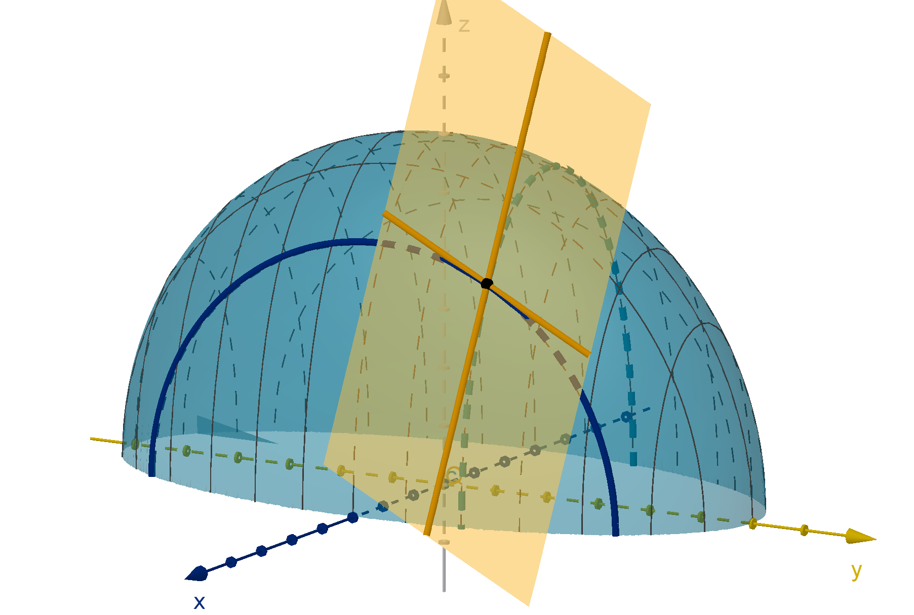
Figure: Tangent lines must have slope 0 at a local max.
This argument works anywhere that ∇f exists. That motivates the following definition:
Definition
We say P is a critical point of f if either
1 ∇f(P ) =
0 or
2 ∇f(P ) does not exist (because one of the partial derivatives does not exist).
Theorem
The local maximums and minimums of a function can only occur at critical points.
Example 5.6.3
Finding Critical Points
The function z = 2x
2
+ 4x + y
2
− 6y + 13 has a minimum value. Find it.
376
Solution
We know the minimum value exists, so it must lie at a critical point. We compute
∇f(x, y) = ⟨4x + 4, 2y − 6⟩
One type of critical point is where this is undefined, but no value of (x, y) makes these expressions
undefined. The other type of critical point occurs when these components are 0. We can solve that
system of equations.
4x + 4 = 0 2y − 6 = 0
x = −1 y = 3
The only point that satisfies this requirement is (−1, 3). Since there is only one critical point, and the
promised minimum lies at a critical point, (−1, 3) must be that point. The minimum value is
z = (2)(−1)
2
+ (4)(−1) + 3
2
− (6)(3) + 13 = 2
¿
Question 5.6.4
How Do We Identify Two-Variable Local Maximums and Minimums?
Once we have found a critical point, how do we know whether it is a local minimum, a local maximum
or neither? Consider a function f(x, y) and a critical point P . There are two possibilities for ∇f(P ). In
the case that ∇f(P ) does not exist, calculus can be no further use to us. If ∇f(P ) = ⟨0, 0⟩, there are
a few different shapes the graph could take. Since we are working with two-variables, we can visualize
these shapes.
A critical point could be a local maximum. In this case f curves downward in every direction.
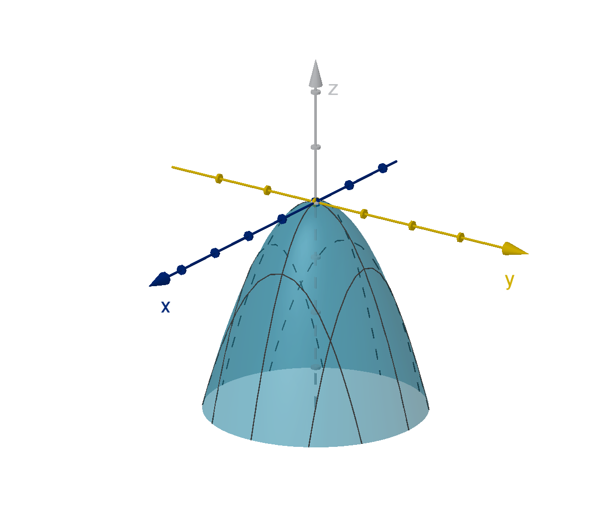
Figure: A local maximum at (0, 0)
377
Question 5.6.4
How Do We Identify Two-Variable Local Maximums and Minimums?
A critical point could be a local minimum. In this case f curves upward in every direction.
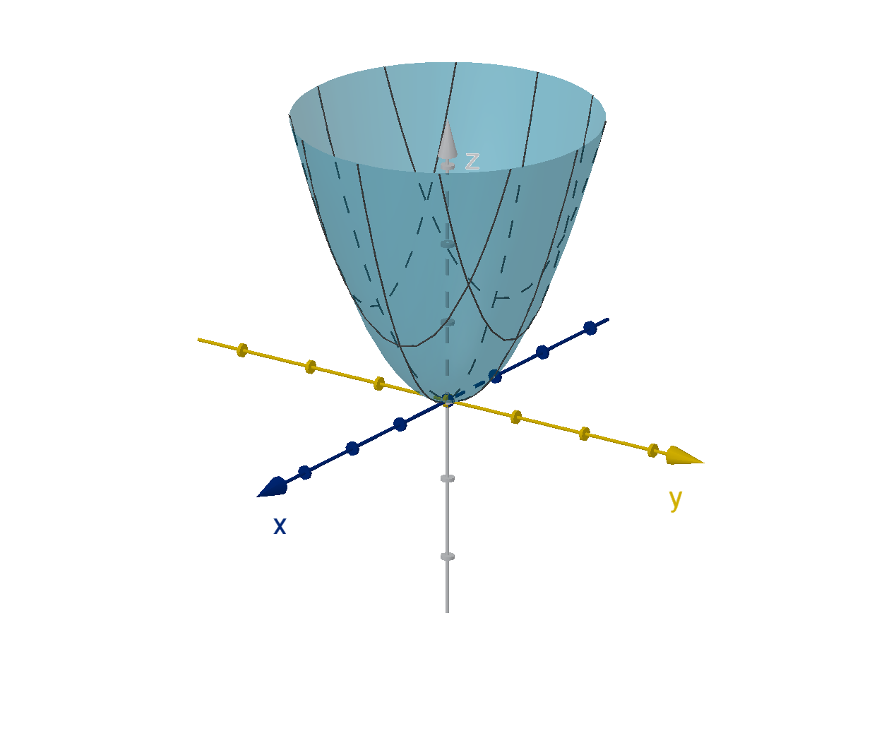
Figure: A local minimum at (0, 0)
A critical point could be neither. f curves upward in some directions but downward in others. This
configuration is called a saddle point.
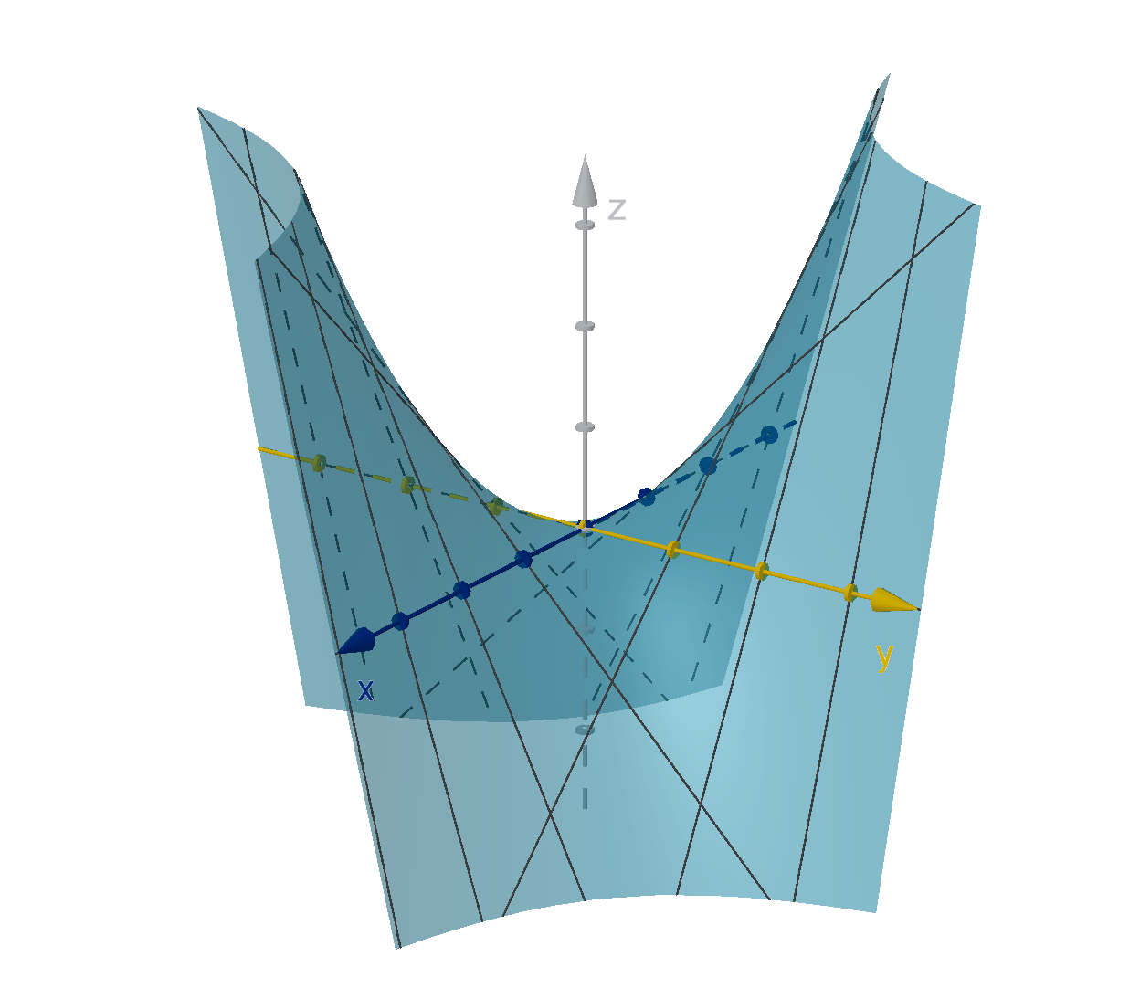
Figure: A saddle point at (0, 0)
Curvature is measured by the second derivatives. This matches our experience with single-variable
critical points, where the second derivative test classifies critical points as local maximums or local
minimums. We have a similar test for two-variable functions, though the computation is more involved.
378
Theorem [The Second Derivatives Test]
Suppose f is differentiable at (P ) and f
x
(P ) = f
y
(P ) = 0. Then we can compute
D = f
xx
(P )f
yy
(P ) − [f
xy
(P )]
2
1 If D > 0 and f
xx
(P ) > 0 then P is a local minimum.
2 If D > 0 and f
xx
(P ) < 0 then P is a local maximum.
3 If D < 0 then P is a saddle point.
Unfortunately, if D = 0, this test gives no information.
Definition
The quantity D in the second derivatives test is actually the determinant of a matrix called the Hessian
of f.
f
xx
(P )f
yy
(P ) − [f
xy
(P )]
2
= det
f
xx
(P ) f
xy
(P )
f
yx
(P ) f
yy
(P )
| {z }
Hf(P )
Hf follows a logical pattern and can be a useful mnemonic for the second derivatives test.
Example 5.6.5
Classifying a Critical Point
Let f(x, y) = cos(2x + y) + xy
a
Verify that ∇f(0, 0) = ⟨0, 0⟩.
b
Is (0, 0) a local minimum, a local maximum, or neither?
379
Example 5.6.5
Classifying a Critical Point
Solution
a
f
x
(x, y) = −sin(2x + y)(2) + y (chain rule)
f
x
(0, 0) = −sin((2)(0) + 0)(2) + 0 = 0
f
y
(x, y) = −sin(2x + y)(1) + x (chain rule)
f
y
(0, 0) = −sin((2)(0) + 0)(1) + 0 = 0
∇f(0, 0) = ⟨0, 0⟩
b
For the second derivatives test, we need to compute f
xx
, f
xy
and f
yy
at (0, 0).
f
xx
(x, y) = −2 cos(2x + y)(2) (chain rule)
f
xx
(0, 0) = −2 cos((2)(0) + (0))(2) = −4
f
xy
(x, y) = −2 cos(2x + y)(1) + 1 (chain rule)
f
xy
(0, 0) = −2 cos((2)(0) + (0))(1) + 1 = −1
f
yy
(x, y) = −cos(2x + y)(1) (chain rule)
f
yy
(0, 0) = −cos((2)(0) + (0))(1) = −1
D = f
xx
(0, 0)f
yy
(0, 0) − [f
xy
(0, 0)]
2
= (−4)(−1) − (−1)
2
= 3
Since D > 0 and f
xx
< 0, (0, 0) is a local maximum of f.
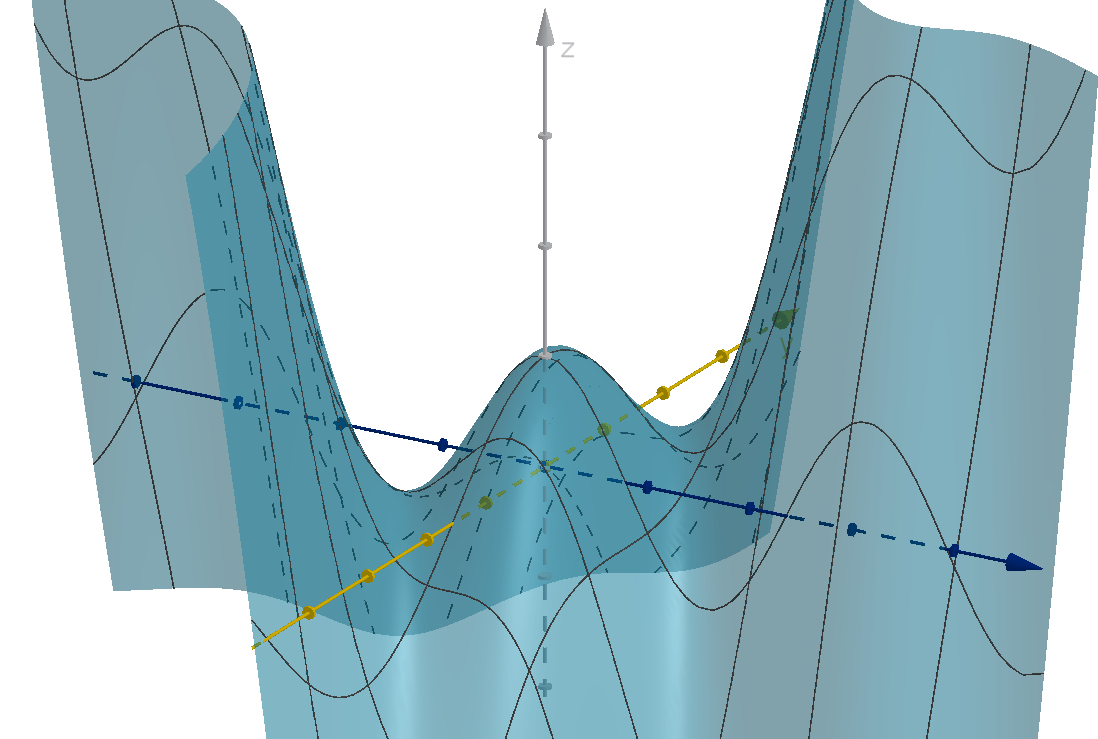
Figure: The graph z = cos(2x + y) + xy with a local maximum at (0, 0)
380
Remark
Why does the final determination between maximum and minimum rely on f
xx
(P ) instead of f
yy
(P )?
Actually it doesn’t matter which we test. In order for D to be positive, f
xx
(P ) and f
yy
(P ) must have
the same sign.
Question 5.6.6
How Do We Find Global Extremes?
The second derivatives test can categorize local extremes, but what about a global extreme?
Definition
Given an n-variable function f (x
1
, x
2
, . . . , x
n
) we say that a point P in n-space is
1 a local maximum if f(P ) ≥ f(Q) for all Q in the domain of f.
2 a local minimum if f(P ) ≤ f(Q) for all Q in the domain of f.
In a real-world application, we are much more interested in finding global extremes than local ones.
Many abstract functions do not even have global extremes. y = e
x
has no global maximum. It increases
without bound. y =
1
x
2
has no global minimum. It approaches 0 but never reaches it. The following
theorem guarantees that certain functions will have global extremes for us to try to find.
Theorem [The Extreme Value Theorem]
A continuous function f on a closed and bounded domain D has a global maximum and a global
minimum somewhere in D.
Two of the words in this theorem have not been defined yet. Here are their definitions.
Definition
Let D be a subset of n-space.
D is closed if it contains all of the points on its boundary.
D is bounded if there is some upper limit to how far its points get from the origin (or any other
fixed point). If there are points of D arbitrarily far from the origin, then D is unbounded.
381
Question 5.6.6
How Do We Find Global Extremes?
For one-variable functions. The EVT requires that the domain be a union of finite, closed intervals
(and maybe finitely many isolated points).
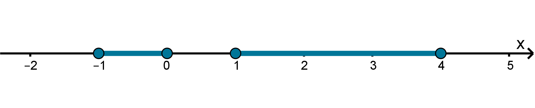
Figure: A union of finite, closed intervals
In 2-space, we can get a better sense of what these requirements mean. The boundary of D is
the set of points from which you can find points in D and points outside D arbitrarily close by. The
boundary of a disc is a circle. If the disc includes the circle, it is closed. If it does not include the circle,
it is not closed.
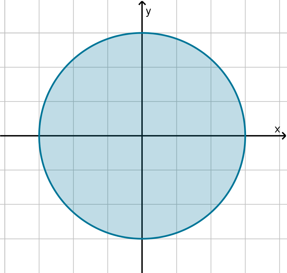
Figure: x
2
+ y
2
≤ 9 is closed.
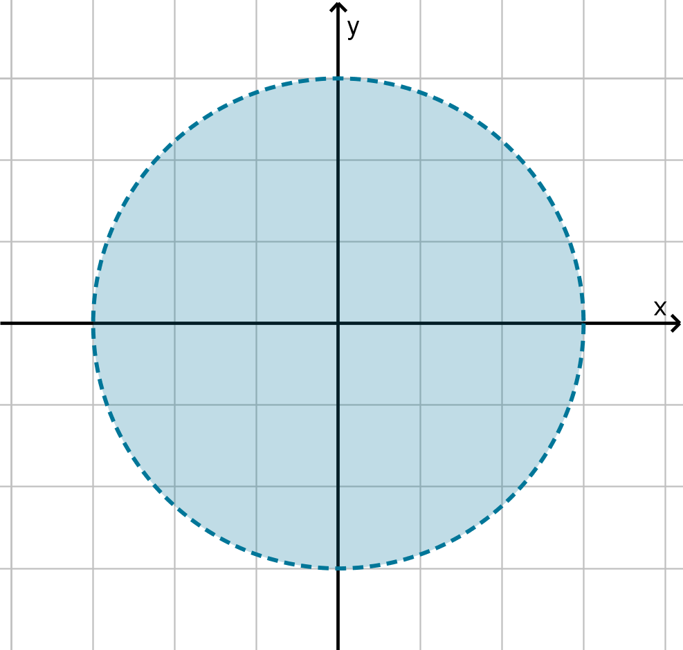
Figure: x
2
+ y
2
< 9 is not closed.
Containing part of the boundary is not enough. Any missing point means that D is not closed. Even
removing an isolated point from the interior of D is a problem. That point is arbitrarily close to points
in D. It is also arbitrarily close to a point outside D, itself. Thus it is a boundary point not contained
in D, and D is not closed.
382
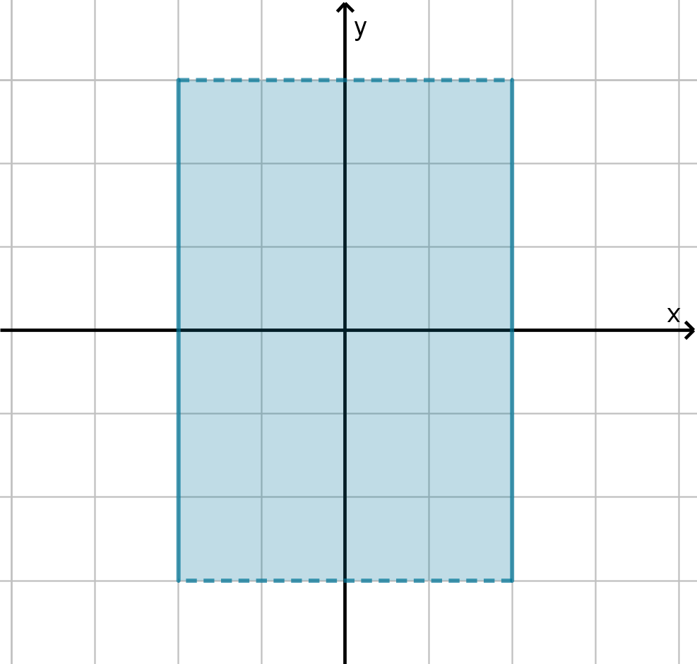
Figure: −2 ≤ x ≤ 2 and −3 < y < 3 is
not closed.
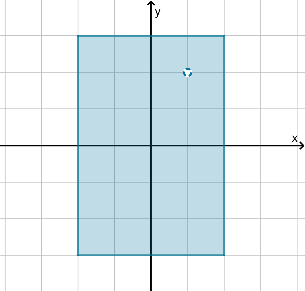
Figure: −2 ≤ x ≤ 2 and −3 ≤ y ≤ 3
and (x, y) = (1, 2) is not closed.
Bounded regions are easier to understand. If we can enclose the region in a sufficiently large circle,
it is bounded. If it stretches outside any circle we would draw around it, then it is unbounded.
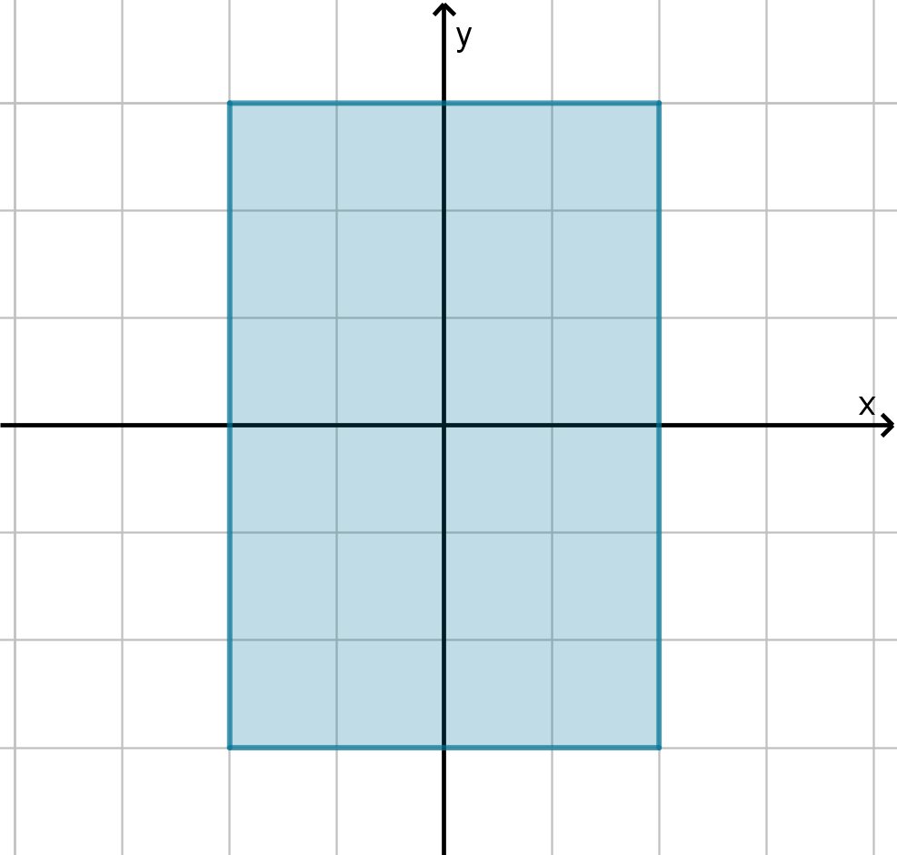
Figure: −2 ≤ x ≤ 2 and −3 ≤ y ≤ 3 is
bounded.
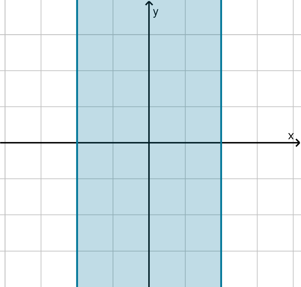
Figure: −2 ≤ x ≤ 2 is unbounded.
Example 5.6.7
Finding a Global Maximum
Consider the function f (x, y) = x
2
+ 2y
2
− x
2
y on the domain
D = { (x, y)
|{z}
points in R
2
: x
2
+ y
2
≤ 16, x ≤ 0
| {z }
conditions
}
a
Does f have a maximum value on D? How do we know?
383
Example 5.6.7
Finding a Global Maximum
b
Find the critical points of f .
c
Must one of the critical points be the maximum?
d
Find the maximum of f .
Remark
The set notation
{type of objects in the set : conditions that thoise objects must satisfy}
is used throughout mathematics, because it is so flexible. It can denote sets of numbers, points,
functions, vectors or any other objects.
Solution
a
f is a polynomial, so it is continuous. D is a semi-disc that includes its boundary, so it is closed
and bounded. The extreme value theorem guarantees that f has a global maximum on D.
b
We begin by computing the gradient of f.
f
x
(x, y) = 2x − 2xy f
y
(x, y) = 4y − x
2
384
These are never undefined, so there are no critical points of that type. The only critical points
will be where both partial derivatives are 0.
0 = 2x − 2xy 0 = 4y − x
2
0 = 2x(1 − y) (factor 2x − 2xy)
x = 0 or y = 1
0 = 4y − 0
2
0 = 4(1) − x
2
(examine each case seperately)
0 = y x = ±2
We should be careful not to lose track of the logic. The x = ±2 solution goes with the y = 1
case. The y = 0 solution goes with the x = 0 case. Mixing these up will give invalid solutions.
You can always plug in pair of (x, y) to verify they satisfy the system of equations.
We conclude that (0, 0), (2, 1) and (−2, 1) are the critical points, but (2, 1) is not in the domain,
so we discard it.
c
No. Recall our method for maximizing single variable functions on a closed interval. The maximum
can occur at the endpoint of the interval without being detected by the derivative.
The same is true here. If the maximum is on the boundary of D, the gradient need not be 0. In
the single-variable case, we only need to test the endpoints (by evaluating f there). There are
infinitely many points on the boundary of D. Evaluating f on all of them is not an option. With
graphing software we can see that the maximum occurs on the boundary somewhere in the third
quadrant, but how can we solve for it exactly?
385
Example 5.6.7
Finding a Global Maximum
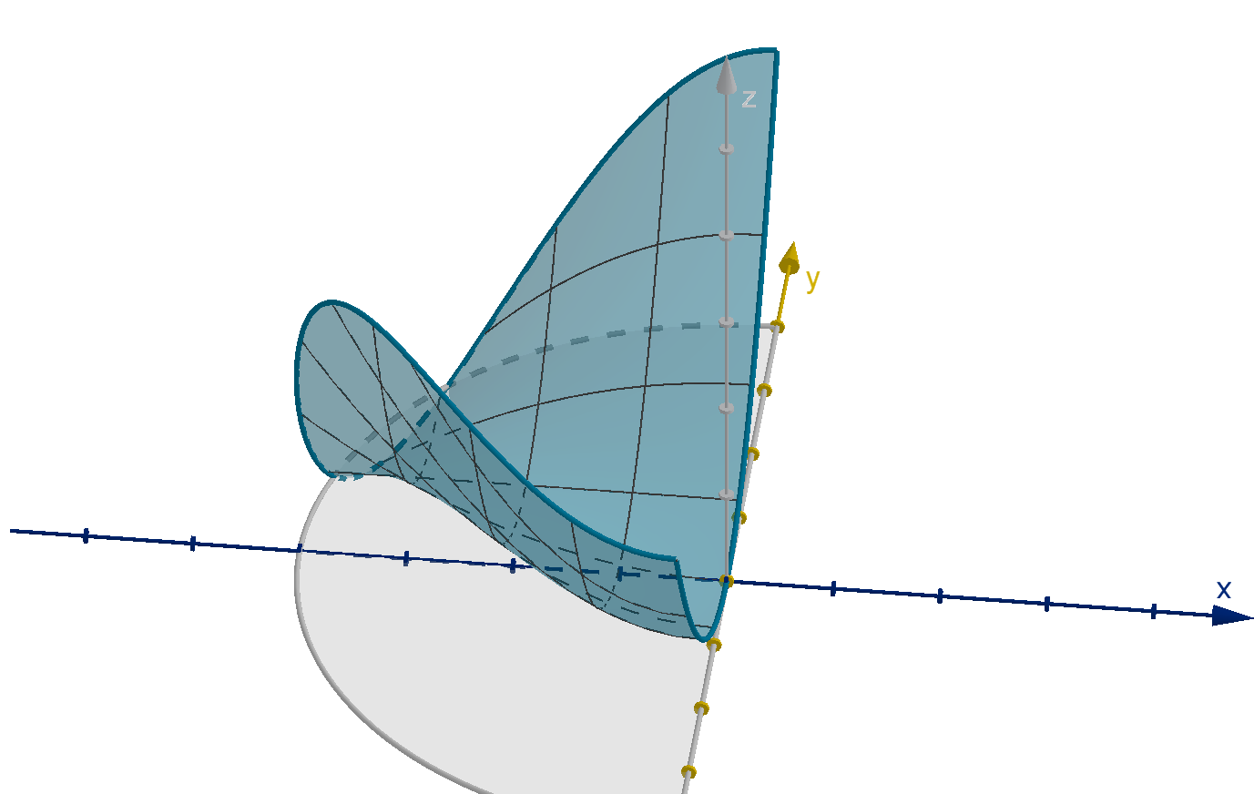
Figure: The graph of y = f(x, y) over the domain D
d
To narrow down the search for a maximum on the boundary of D, we will use the boundary
equations to write an expression for f that is valid only on the boundary. We can find the critical
points of this expression, and rule out any point that is not a critical point.
Suppose the maximum lies on x = 0. The function on x = 0 is f(0, y) = 0
2
+ 2y
2
− 0
2
y =
2y
2
. This function only has one variable, so we can find potential maximums by looking for
its critical points.
f
′
(y) = 4y
This is never undefined. It is 0 at y = 0. The only critical point of f (y) on x = 0 is (0, 0).
However, not all of x = 0 is the boundary of D. This component of the boundary ends
at (0, 4) and (0, −4). Like with a closed interval, the derivative of f(y) cannot detect a
maximum at those endpoints.
Suppose the maximum lies on x
2
+ y
2
= 16. On this graph, we can similarly reduce f(x, y)
to a function of one variable, but the substitution is more complicated. We solve
x
2
+ y
2
= 16
x
2
= 16 − y
2
f(y) = (16 − y
2
) + 2y
2
− (16 − y
2
)y (substitute for x
2
)
= y
3
+ y
2
− 16y + 16
f
′
(y) = 3y
2
+ 2y − 16
0 = 3y
2
+ 2y − 16 (solve for critical points)
0 = (3y + 8)(y − 2)
y = −
8
3
y = 2
x
2
+
−
8
3
2
= 16 x
2
+ 2
2
= 16 (substituue into x
2
+ y
2
= 16)
x
2
= 16 −
64
9
x
2
= 16 − 4
386
x = −
r
80
9
x = −
√
12 (+ solutions are not in D)
Our critical points are
−
q
80
9
, −
8
3
and
−
√
12, 2
. This component of the boundary also
ends at (0, 4) and (0, −4), so the maximum might lie there.
We can now argue that one of the points we have found is the maximum.
If the maximum is not on the boundary, it lies at (−2, 1).
If the maximum is on x = 0, then it lies at (0, 0), (0, 4) or (0, −4).
If the maximum is on x
2
+ y
2
= 16, then it lies at
−
q
80
9
, −
8
3
,
−
√
12, 2
, (0, 4) or
(0, −4).
One of these must be the case. To figure out which it is, we can evaluate f at each point and see
which produces the largest value.
f(−2, 1) = (−2)
2
+ 2(1)
2
− (−2)
2
(1) = 2
f(0, 0) = (0)
2
+ 2(0)
2
− (0)
2
(0) = 0
f(0, 4) = (0)
2
+ 2(4)
2
− (0)
2
(4) = 32
f(0, −4) = (0)
2
+ 2(−4)
2
− (0)
2
(−4) = 32
f
−
q
80
9
, −
8
3
=
−
q
80
9
2
+ 2
−
8
3
2
−
−
q
80
9
2
−
8
3
=
1264
27
(maximum)
f
−
√
12, 2
= (−
√
12)
2
+ 2(2)
2
− (−
√
12)
2
(2) = −4
Main Ideas
If the Extreme Value Theorem applies, then all we need to do is find the critical points and evaluate
f at each. One is guaranteed to be the maximum, and one is guaranteed to be the minimum.
∇f =
0 will detect critical points on the interior, but not on the boundary.
We can rewrite the function on a boundary component using substitution. Set the derivative equal
to 0 to find critical points.
Derivatives will not detect maximums at the endpoints of a boundary curve. These must be
included in your set of critical points.
387
Section 5.6
Exercises
Summary Questions
Q1
Where must the local maximums and minimums of a function occur? Why does this make sense?
Q2
What does the second derivatives test tell us?
Q3
What hypotheses does the Extreme Value Theorem require? What does it tell us?
Q4
Assuming a maximum and minimum exist, where must you look in a domain to be sure you find
them?
5.6.1
Q5
Raina claims that (0, 0) is the maximum of f (x, y) = x
2
−y
2
−10xy. Disprove her claim without
using calculus.
Q6
Is a global maximum also a local maximum? Explain.
Q7
Suppose g(x, y) = e
f(x,y)
. If (a, b) is a local minimum of f(x, y), is it also a local minimum of
g(x, y)? Explain.
Q8
Does a constant function have any local maximums? Justify your answer with the definition of
local maximum.
388
5.6.2
Q9
Suppose ∇f(4, 2) = ⟨−5, 11⟩. Where would you travel from (4, 2) to find higher values of f?
Q10
The function f (x, y) = |x|+|y| has its global minimum at (0, 0). Is this a critical point? Explain.
Q11
If (a, b) produces the minimum value of |∇f(x, y)|, must (0, 0) must be a critical point? Explain.
Q12
Suppose f(x) is a function of x with critical points x = a and x = b. Suppose g(y) is a function
of y with critical points y = c and y = d. What are the critical points of h(x, y) = f(x) +g(y)?
5.6.3
Q13
Find the critical points of f (x, y) = x
4
+ 4xy + y
4
.
Q14
Find the critical points of g(x, y) = x
2
+ y
2
− 3xy − 13x + 12y.
5.6.4
Q15
If (x
0
, y
0
) is critical point and f
(
xx)(x
0
, y
0
) = 0, can (x
0
, y
0
) be a local maximum of f ? What
must be the value of f
xy
(x
0
, y
0
) if so?
Q16
For what values of a does f(x, y) = x
2
+ y
2
+ axy have a local minimum at the origin?
389
Section 5.6
Exercises
5.6.5
Q17
Find the critical points of h(x, y) = x
2
y − x
2
− 2y
2
. Classify each as a local maximum, local
minimum, or saddle point.
Q18
Find all critical points of f(x, y) =
1
3
x
3
− 4xy + 2y
2
. Classify them as local maximums, local
minimums, or saddle points.
Q19
Compute the critical points of f(x, y) = 2x
3
−12xy + 3y
2
and classify each as a local maximum,
local minimum, or saddle point.
Q20
Let h(x, y) = x
2
+ y
3
+ 3xy. Find the critical points of h, and classify each as a local maximum,
local minimum or saddle point.
Q21
Let f(x, y) = x
3
−15x
2
−9x + 12xy −3y
2
−18y. Find the critical points of f and classify each
one as local maximum, local minimum or saddle point.
Q22
Let f(x, y) = x
5
+ 20xy + 5y
2
. Find the critical points of f and classify each one as local
maximum, local minimum or saddle point.
Q23
Find the critical points of g(x, y) = e
x
3
+y
2
−12x+10y
. Classify each one as local maximum, local
minimum or saddle point.
Q24
Find the critical points of f(x, y) =
1
x
4
−x
2
y+y
2
+10
. Classify each one as local maximum, local
minimum or saddle point.
5.6.6
Q25
Draw a sketch of D = {(x, y) : y ≥ x
2
, y ≤ x
3
}. State whether D is closed and whether D is
bounded.
Q26
Draw a sketch of D = {(x, y) : y ≥ x, y ≤ 2x, xy < 1}. State whether D is closed and whether
D is bounded.
Q27
Draw a sketch of D = {(x, y) : x > 0, y ≥ x
4
}. State whether D is closed and whether D is
bounded.
390
Q28
Draw a sketch of D = {(x, y) : − 1 < x
2
+ y
2
≤ 16}. State whether D is closed and whether
D is bounded.
Q29
Let D = {(x, y) : y ≥ x
2
}. Can the Extreme Value Theorem guarantee that f has a maximum
on D? Explain.
Q30
Does the function f (x, y) =
1
x
2
+y
2
have a maximum and minimum value on the domain D =
{(x, y) : −3 ≤ x ≤ 3, −4 ≤ y ≤ 4}? If yes, find them. If not, explain why the extreme value
theorem does not apply.
5.6.7
Q31
Draw a careful diagram of D = {(x, y) : y ≥ x
2
, x
2
+ y
2
≤ 20}. Where would you need to
check to guarantee you’d find the maximum value of a continuous function f on D?
Q32
Let f(x, y) be a differentiable function and let
D = {(x, y) : y ≥ x
2
− 4, x ≥ 0, y ≤ 5}.
a
Sketch the domain D.
b
Does the Extreme Value Theorem guarantee that f has an absolute minimum on D? Explain.
c
List all the places you would need to check in order to locate the minimum.
Q33
Find the maximum and minimum value of f (x, y) = e
x+3y
in the triangle with vertices (0, 0),
(6, 0) and (0, 3).
Q34
Find the maximum and minimum value of f (x, y) = 3x + y on D, the closed region bounded by
y = x
2
and y = 16.
Q35
Find the global max and min of f(x, y) = x
3
− 12x + y
3
− 3y on the rectangle 0 ≤ x ≤ 4 and
−2 ≤ y ≤ 2.
Q36
Consider the function g(x, y) =
x
4
−2x
2
+2
y
2
−2y+2
on the rectangle −2 ≤ x ≤ 2 and 0 ≤ y ≤ 3.
391
Section 5.6
Exercises
a
Does the extreme value theorem apply to this function? Why might you be concerned, and
what would you have to check?
b
Find the min and max of g.
Synthesis and Extension
Q37
Consider the function f (x, y) = x
2
− 4xy + 4y
2
.
a
Find the critical point(s) of f .
b
What does the second derivatives test say about the critical points of f?
c
Can you classify the critical points using algebra instead? Explain.
Q38
If g(x) is an increasing function, explain why the local maximums and minimums of any f(x, y)
are the same as the local maximums and minimums of g(f(x, y)).
392
Section 5.7
Lagrange Multipliers
Goals:
1 Find minimum and maximum values of a function subject to a constraint.
2 If necessary, use Lagrange multipliers.
Many of the functions we studied do not have maximum values. Polynomials and exponential
functions increase without bound. Yet in the real world, we never see corporations producing infinite
quantities of goods. We never see infinite populations of animals. Does this mean that polyonomials and
exponentials have no real-world applications? On the contrary, they are ubiquitous, but the corporations
and populations that opperate under these models also have constraints on their inputs.
Corporations do not have infinite money to invest. Animals do not have infinite food sources. In
this section we develop the tools to find maximum and minimum values of a function, when our inputs
are constrained.
Question 5.7.1
What Is a Constraint?
Sometimes we aren’t interested in the maximum value of f(x, y) over the whole domain, we want
to restrict to only those points that satisfy a certain constraint equation.
The maximum on the constraint is unlikely to
be the same as the unconstrained maximum
(where ∇f = 0). Can we still use ∇f to find
the maximum on the constraint?
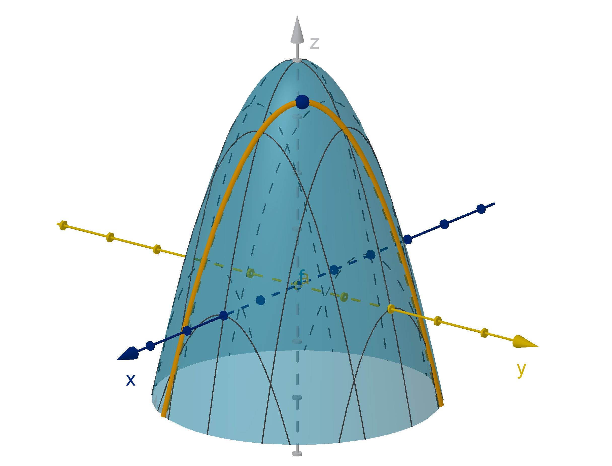
Figure: Maximizing f such that x + y = 1
We explore this question in the Maximums on a Constraint activity.
Question 5.7.2
How Do We Solve a Constrained Optimization?
The method of Lagrange Multipliers makes use of the following theorem.
393
Question 5.7.2
How Do We Solve a Constrained Optimization?
Theorem
Suppose an objective function f(x, y) and a constraint function g(x, y) are differentiable. The local
extremes of f(x, y) given the constraint g(x, y) = c occur where
∇f = λ∇g
for some number λ, or else where ∇g = 0. The number λ is called a Lagrange Multiplier.
This theorem generalizes to functions of more variables.
We can justify the theorem visually by examining the relationship ∇f, ∇g and the constraint. The
constraint g(x, y) = c is by definition a level curve of g. It is normal to ∇g.
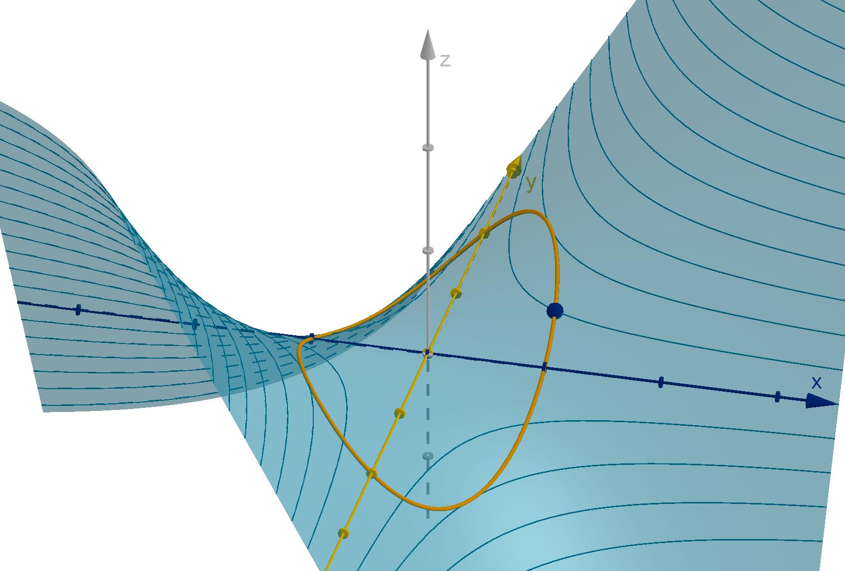
Figure: Where ∇f is not parallel to ∇g, we can travel along g(x, y) = c and increase the value of f .
This is because D
u
f > 0 for some u along the constraint.
By this argument, the only place a maximum or minimum of the objective function can lie of the
contraint is where D
u
f would have to be 0, because ∇f is parallel to ∇g.
Remark
When ∇f(P ) is parallel to ∇g(P ) (and neither of these vectors is
0), the level curves of f through P
is tangent to the level curve g(x, y) = c. If we can draw the level curves of f , this gives us a visual
method of identifying the potential maximums and minimums.
Example 5.7.3
The Maximum on a Curve
Find the point(s) on the ellipse 4x
2
+ y
2
= 4 on which the function f (x, y) = xy is maximized.
394
The EVT and constraints
Are we guaranteed that a maximum exists at all? The Extreme Value Theorem can still be applied to
constraints. Here are a few ways we can identify that a constraint is closed:
1 A curve is closed if it includes its endpoints (or none exist).
2 A surface is closed if it includes its boundary (or none exists).
3 The level set of a continuous function is always closed.
Even armed with these, we still need to check that the domain is bounded.
Solution
We’ll check the conditions of the Extreme Value Theorem
1 4x
2
+ y
2
= 4 is a curve with no endpoints, so it is closed.
2 4x
2
+ y
2
= 4 is an ellipse. It stays within a bounded distance from the origin.
3 f is continuous.
By the Extreme Value Theorem, we know that a maximum exists. We will use Lagrange multipliers
to narrow down our search to the possible maximums. We set g(x, y) = 4x
2
+ y
2
and compute the
gradient vectors of f and g.
∇f(x, y) = ⟨y, x⟩ ∇g(x, y) = ⟨8x, 2y⟩
The theorem allows two possibilities at a maximum.
1 ∇g(x, y) = ⟨0, 0⟩. The only (x, y) that satisfies this is (0, 0). But (0, 0) is not on the constraint,
so it is not a valid solution.
2 ∇f = λ∇g. We can factor the λ across each component of the vectors, but that gives us two
equations and three variables (x ,y and λ). We need another equation, and fortunately we have
one. x and y must satisfy 4x
2
+ y
2
= 4 as well. Here is one (but not the only) way to solve this
system of equations.
395
Example 5.7.3
The Maximum on a Curve
y = λ8x x = λ2y 4x
2
+ y
2
= 4
y = λ8(λ2y)
0 = λ
2
16y − y
0 = y(4λ − 1)(4λ + 1)
either 0 = y x = λ2(0) 4(0)
2
+ 0
2
= 4 (no solution)
or λ = ±
1
4
y =
±
1
4
8x
y = ±2x
4x
2
+ (±2x)
2
= 4
8x
2
= 4
x
2
=
1
2
x = ±
1
√
2
y = ±2
1
√
2
y = ±
√
2
This tells us the only possible locations for the maximum are:
(x, y) =
±
1
√
2
, ±
√
2
We identify the maximum by evaluating f at each point.
f
1
√
2
,
√
2
= 1 f
−
1
√
2
,
√
2
= −1
f
−
1
√
2
, −
√
2
= 1 f
1
√
2
, −
√
2
= −1
We conclude that the maximum occurs at
1
√
2
,
√
2
and
−
1
√
2
, −
√
2
.
396
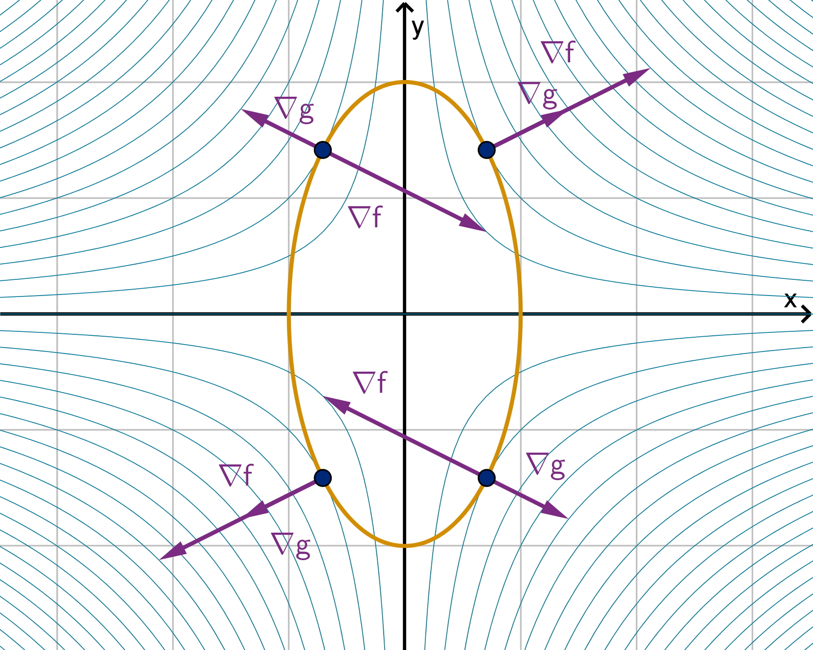
Figure: The four points that satisfy ∇f = λ∇g and g(x, y) = c.
Main Idea
The level set of a continuous (constraint) function is always closed. If it is also bounded and the
objective function is differentiable, then one of the points produced by Lagrange multipliers will be the
global maximum and one will be the global minimum of the constrained optimization.
Example 5.7.4
The Maximum on a Surface
Find the maximum value of the function f(x, y, z) = x
4
y
4
z on the sphere x
2
+ y
2
+ z
2
= 36.
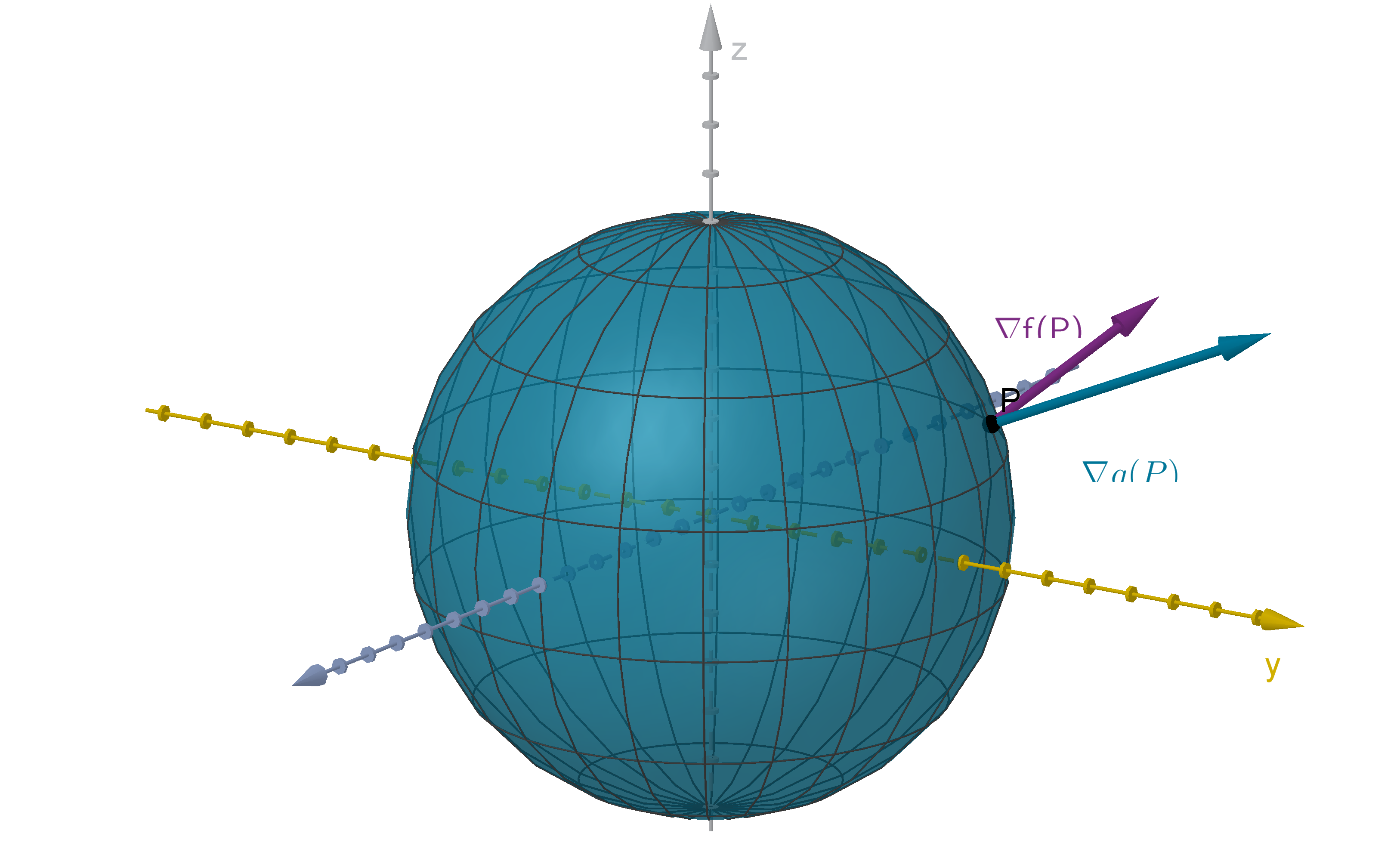
Figure: The gradient vector and level surface of a constraint function and the gradient vector of the
objective function
397
Example 5.7.4
The Maximum on a Surface
Solution
First note that the EVT applies, since a sphere is closed and bounded and f is continuous. To identify
potential maximums, we appeal to Lagrange multipliers.
Set g(x, y, z) = x
2
+y
2
+z
2
. Then ∇g(x, y, z) = ⟨2x, 2y, 2z⟩. The case ∇g(x, y, z) =
0 only occurs
at the origin, which is not on the sphere. The critical points must be only the points where ∇f = λ∇g.
∇f(x, y, z) =
4x
3
y
4
z, 4x
4
y
3
z, x
4
y
4
.
Equating each coordinate gives us three equations, and the constraint is a fourth. We thus have a
system of four equations and four variables.
4x
3
y
4
z = λ2x 4x
4
y
3
z = λ2y x
4
y
4
z = λ2z x
2
+ y
2
+ z
2
= 36
The most obvious way to solve this algebraically is to solve for λ, but this requires us to divide by
x, y and z. We would need to remember that another possible solution is that x, y or z is 0. We can
avoid this by multiplying and factoring instead.
4x
3
y
4
z = λ2x 4x
4
y
3
z = λ2y x
4
y
4
= λ2z
4x
3
y
5
z
2
= λ2xyz 4x
5
y
3
z
2
= λ2xyz x
5
y
5
= λ2xyz
4x
3
y
5
z
2
= 4x
5
y
3
z
2
x
5
y
5
= 4x
5
y
3
z
2
4x
3
y
5
z
2
− 4x
5
y
3
z
2
= 0 x
5
y
5
− 4x
5
y
3
z
2
= 0
4x
3
y
3
z
2
(y − x)(y + x) = 0 x
5
y
3
(y − 2z)(y + 2z) = 0
either x = 0
or y = 0
or y = ±x and y = ±2z
±2z = x
x
2
+ y
2
+ z
2
= 36
(±2z)
2
+ (±2z)
2
+ z
2
= 36
9z
2
= 36
z = ±2
(±2)(±2) = x y = (±2)(±2)
±4 = x y = ±4
This gives us 8 critical points: (±4, ±4, ±2). In addition every point in the x = 0 cross section of
the sphere is a critical point, as is every point in the y = 0 cross-section. This is infinitely many points
to evaluate, but fortunately the algebra of our objective function allows us to evaluate these points in
large batches.
if x = 0 f (x, y, z) = 0
4
y
4
z = 0
if y = 0 f (x, y, z) = x
4
0
4
z = 0
f(±4, ±4, 2) = (±4)
4
(±4)
4
(2) = 2
17
f(±4, ±4, −2) = (±4)
4
(±4)
4
(−2) = −2
17
Thus the maximum value is 2
17
. It occurs at the four points (±4, ±4, 2).
398
Remark
If we hadn’t seen how to avoid dividing by x, y and z, we could have gone ahead and done the division.
Remember that when you divide while solving an equation, you obtain an extra solution where the divisor
is 0. This would lead us to check x = 0, y = 0 and z = 0 as we did in the factoring solution.
Synthesis 5.7.5
Using the Extreme Value Theorem and Lagrange Multipliers
How can Lagrange multipliers help us find the maximum of f(x, y) = x
2
+ 2y
2
−x
2
y on the domain
D = {(x, y) : x
2
+ y
2
≤ 16, x ≤ 0}?
Solution
We can continue Example 7. After finding the critical points of f at (0, 0) and (−2, 1), we turn to the
boundaries. The boundaries are level curves.
For x
2
+ y
2
= 16, set g(x, y) = x
2
+ y
2
= 16. We have
∇f(x, y) =
2x − 2xy, 4y − x
2
∇g(x, y) = ⟨2x, 2y⟩
∇g(x, y) =
0 only at the origin, which isn’t on the constraint. So we solve ∇f(x, y) = λ∇g(x, y)
and g(x, y) = 4.
399
Synthesis 5.7.5
Using the Extreme Value Theorem and Lagrange Multipliers
2x − 2xy = λ2x 4y − x
2
= λ2y x
2
+ y
2
= 16
2x − 2xy − 2λx = 0
2x(1 − y − λ) = 0
if x = 0 0
2
+ y
2
= 16
y = ±4
if 1 − y − λ = 0
λ = 1 − y 4y − x
2
= (1 − y)2y
2y
2
+ 2y = x
2
(2y
2
+ 2y) + y
2
= 16
3y
2
+ 2y − 16 = 0
(3y + 8)(y − 2) = 0
if y = −
8
3
if y = 2
x
2
+
−
8
3
2
= 16 x
2
+ 2
2
= 16
x
2
+
64
9
=
144
9
x
2
= 12
x
2
=
80
9
= x = ±
√
12
x = ±
r
80
9
The critical points are (0, ±4),
−
√
12, 2
and
−
q
80
9
, −
8
3
. The solutions with positive x are
not in D.
On x = 0, substitution is probably the easier choice, but Lagrange multipliers are still possible.
x = 0 is a level set of the function g(x, y) = x.
∇g(x, y) = ⟨1, 0⟩
∇g =
0 so we solve ∇f (x, y) = λ∇g(x, y).
2x − 2xy = λ 4y − x
2
= 0 x = 0
4y = 0
This is the same equation we obtained by substituting x = 0 into f and differentiating.
400
Main Idea
To find the absolute minimum and maximum of a differentiable function f(x, y) over a closed and
bounded domain D:
1 Compute ∇f and find the critical points inside D.
2 Identify the boundary components. Find the critical points on each using substitution or Lagrange
multipliers.
3 Identify the endpoints (intersections) of the boundary components.
4 Evaluate f(x, y) at all of the above. The minimum is the lowest number, the maximum is the
highest.
Synthesis 5.7.6
The Gradient on the Boundary
Suppose P is a critical point of f on a boundary component of a domain D. What does the direction
of ∇f(P ) tell us about whether P is a maximum or minimum?
Figure: The critical points and gradient vectors of f(x, y) on a closed and bounded domain
Solution
First suppose ∇f(P ) points into D. Then f increases as we travel into D. Thus P cannot be a local
maximum.
401
Synthesis 5.7.6
The Gradient on the Boundary
P may be a local minimum but may not be. The directional derivative along the boundary is 0, so f
could curve upward or downward along the boundary. If f curves downward we could find lower values
of f nearby and P would not be a minimum. If f curves upward, then P would be a minimum. We
could compute this curvature by taking the substituted version of f that we used to solve for P and
computing its second derivative at P .
On the other hand, if we suppose that ∇f(P ) points out of D, then D decreases as we travel into
D, and P cannot be a local minimum. It may or may not be a local maximum.
Question 5.7.7
Can This Lagrange Apply to More Than One Constraint?
If we have two constraints in three-space, g(x, y, z) = c and h(x, y, z) = d, then their intersection
is generally a curve.
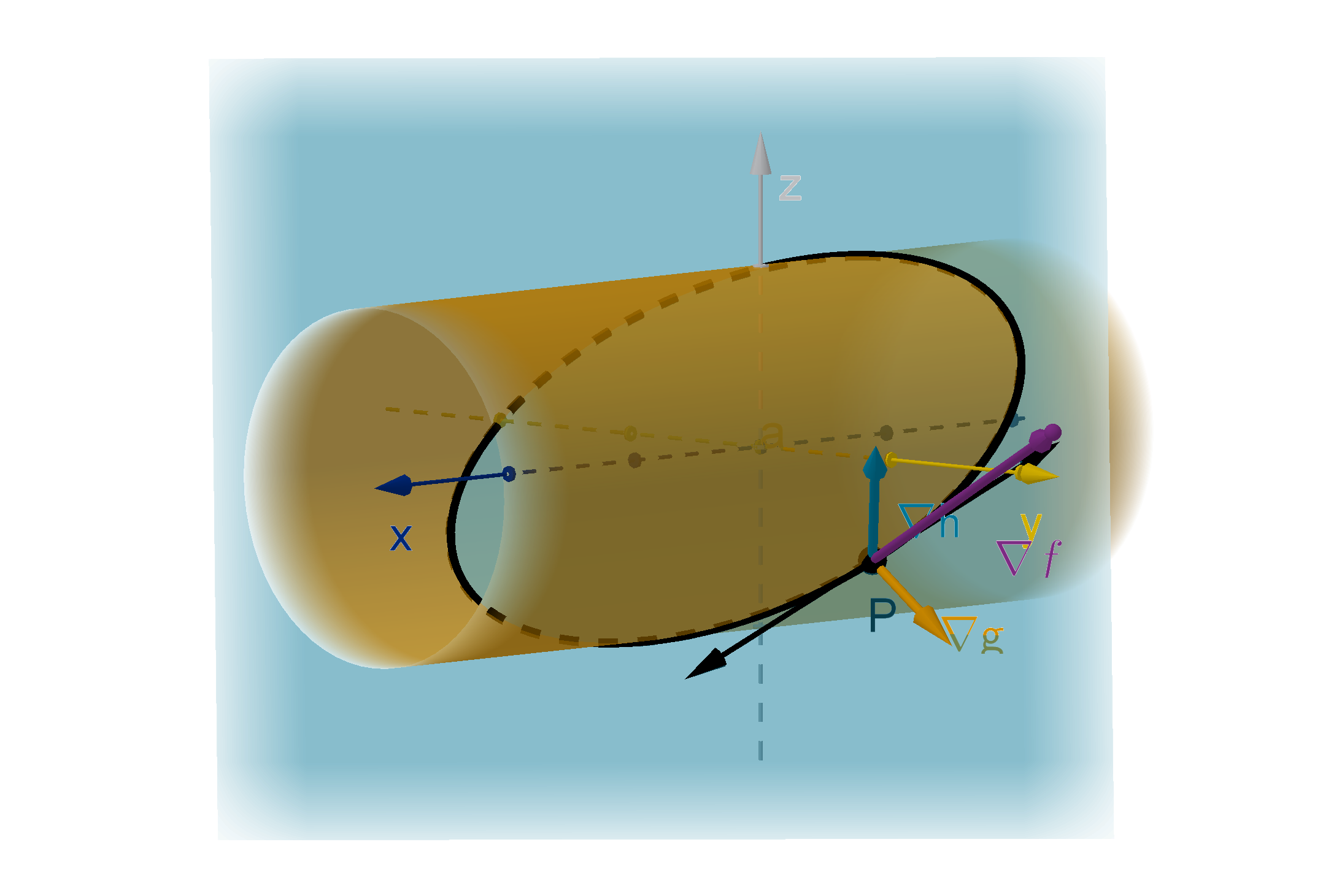
Figure: The intersection of the constraints g(x, y, z) = c and h(x, y, z) = d
According to our earlier argument about directional derivatives, at a maximum P on the constraint,
∇f(P ) must be normal to the constraint. There are more ways for this to happen with two constraint
equations.
1 ∇f(P ) could be parallel to ∇g(P ).
2 ∇f(P ) could be parallel to ∇h(P ).
3 ∇f(P ) could be the vector sum of a vector parallel to ∇g(P ) and a vector parallel to ∇h(P ).
You should look at Figure 380 to convince yourself that these ∇f(P ) would all be normal to the
constraint. We can express this condition algebraically
402
Theorem
If f(x, y, z) is a differentiable function and g(x, y, z) = c and h(x, y, z) = d are two constraints. If P is
a maximum of f (x, y, z) among the points that satisfy these constraints then either
∇f(P ) = λ∇g(P) + µ∇h(P )
for some scalars λ and µ, or ∇g(P) and ∇h(P ) are parallel.
This system of equations is usually difficult to solve by hand.
Remark
You can check the reasonableness of this method by noting that it gives us a system of 5 variables, x,
y, z, λ, µ, and five equations:
f
x
(x, y, z) = λg
x
(x, y, z) + µh
x
(x, y, z) g(x, y, z) = c
f
y
(x, y, z) = λg
y
(x, y, z) + µh
y
(x, y, z) h(x, y, z) = d
f
z
(x, y, z) = λg
z
(x, y, z) + µh
z
(x, y, z)
We therefore generally expect this system to have a finite number of solutions, though there are plenty
of counterexamples to this expectation.
Section 5.7
Exercises
Summary Questions
Q1
What is a constraint?
Q2
What equations do you write when you apply the method of Lagrange multipliers?
Q3
Is the set of points that satisfies a constraint closed and bounded? Explain.
Q4
How does a constraint arise when finding the maximum over a closed and bounded domain?
403
Section 5.7
Exercises
5.7.1
Q5
Suppose we have $230 to spend on three goods. Good 1 costs $13 per unit. Good 2 costs $22
per unit. Good 3 costs $11 per unit. Write a budget constraint that expresses what purchases
(x, y, z) of good 1, good 2 and good 3 are possible, if you spend you budget.
Q6
Suppose the maximum value of f (x, y) occurs at (3, −4). Where is the maximum value of f (x, y)
that satisfies the constraint x
2
+ y
2
= 25? Explain.
5.7.2
Q7
Suppose f (x, y, z) is a smooth function. Suppose the maximum value of f on the sphere x
2
+
y
2
+ z
2
= 25 occurs at P . What can you say about ∇f(P ) and the tangent plane to the sphere
at P ?
Q8
Suppose the curve below is the graph of g(x, y) = k. Use methods from calculus to find and
mark the approximate location of the point that maximizes the function f(x, y) = 3y −x subject
to the constraint g(x, y) = k. Justify your reasoning in a few sentences.
Q9
Suppose that (a, b) is a local maximum of the smooth function f(x, y) which also happens to
satisfy the constraint g(a, b) = k.
a
Is (a, b) also a local maximum of f among the points on the constraint? Explain.
b
If we used Lagrange multipliers to detect (a, b), what would we expect λ to be equal to at
that point?
404
Q10
Show that (3, 3) is not a local maximum of f (x, y) = 2x
2
− 4xy + y
2
− 8x on the graph
x
3
+ y
3
= 6xy.
5.7.3
Q11
Compute the maximum value of y − x
2
on the constraint x
2
+ y
2
= 4.
Q12
Refer to your “Maximums on a Constraint” worksheet.
a
What system of equations would you set up to find the critical points of f on the constraint
p(x, y) = c?
b
Can you solve it?
c
Which was easier, using Lagrange or using substitution?
5.7.4
Q13
Find the maximum value of f (x, y, z) = xyz on the sphere x
2
+ y
2
+ z
2
= 36.
Q14
Find the maximum value of f (x, y, z) = xz on the sphere x
2
+ y
2
+ z
2
= 36.
Q15
Find the maximum value of f (x, y, z) = 3y + 2z on the ellipsoid 25x
2
+ y
2
+ 4z
2
= 100.
Q16
The function h(x, y, z) = x
2
+ y
2
+ z
2
has a minimum value on the plane 3x + 5y − 2z = 30.
Compute it.
405
Section 5.7
Exercises
5.7.5
Q17
Suppose f(x, y) is differentiable but has no critical points. Will the method of Lagrange multipliers
detect the maximum value of f in D = {(x, y) : x
2
+ y
2
≤ 49}? Explain.
Q18
Consider the following two questions:
Find the maximum value of f (x, y) that satisfies x
2
+ y
2
≤ 9.
Find the maximum value of f (x, y) that satisfies x
2
+ y
2
= 9.
a
How are the questions different?
b
Which question takes less work to solve? Explain how you know.
c
Do solutions exist to both questions? What additional information would guarantee that
they do?
Q19
Let D = {(x, y) : x
2
+ y
2
≤ 1, x ≥ 0, y ≤ 0}. Find the maximum and minimum values of
f(x, y) = x
2
− y on D.
Q20
Consider the function f(x, y) = x
2
+ 6xy + 9y
2
+ 5. Find the maximum and minimum values of
f on the domain D = {(x, y) : y ≥ x, x ≥ 0, x
2
+ y
2
≤ 10}
Q21
Let D = {(x, y) : x
2
+ y
2
≤ 20, y ≥ −x}. Find the maximum and minimum values of
f(x, y) = x
4
y on D.
Q22
Let D = {(x, y) : x
2
+ y
2
≤ 25, y ≥ x + 1, y ≥ 0}. Find the maximum and minimum values of
f(x, y) = x
3
y
2
on D.
Q23
Let D = {(x, y) : x
2
+ y
2
≤ 20, y ≥ −x}. Find the maximum and minimum values of
f(x, y) = x
4
y on D.
Q24
Let D =
(x, y) :
x
2
16
+
y
2
64
≤ 1, x ≥ 0
. Find the points in D that obtain the maximum and
minimum values of f (x, y) = 2x + 3y.
406
5.7.6
Q25
Suppose the maximum of f (x, y) on
D = {(x, y) | g(x, y) ≤ c}
occurs at P on the boundary of D. We know that ∇f(P ) points out of D. What does this tell
us about the sign of λ?
Q26
Explain why knowing which way ∇f points is not useful for ruling out potential maximums given
a domain of the form g(x, y) = c.
5.7.7
Q27
How does the method of Lagrange multipliers suggest we solve for the maximum value of f(x, y)
on the constraints x + y = 1 and x −y = 0? Do we need to know what f is to solve this? Why
shouldn’t that bother us?
Q28
Write a system of equations that one would solve to find the maximum and minimum values of
f(x, y, z) = x on the two constraints y
2
+ z
2
= 25 and x + y + z = 1.
Synthesis and Extension
Q29
Consider the plane p with normal equation 7x + 6y − 3z − 42 = 0
a
Use Lagrange multipliers to find the point A on p that s closest to the origin O.
b
Show that
−→
OA is a normal vector to p.
c
Show how you can use the observation in
b
to solve for the closest point (A) without using
calculus.
Q30
Determine the smallest rectangle (parallel to the x and y axes) that contains the ellipse x
2
+
3xy + 4y
2
− 4x − 13y + 4 = 0.
407
Section 5.7
Exercises
Q31
An aquarium with an open top has volume 20m
3
. Its rectangular base is made of slate, and its
sides are made of glass. Slate costs five times as much (per unit area) as glass. Set up and solve
a constrained onstrained optimization problem to find the dimensions (ℓ, w, h) of the aquarium
that will minimize the cost of materials.
Q32
Let D be the region enclosed by 2x + y = 8, y = 8 and x = 4. Consider the function
f(x, y) = xy − 3y − 6x.
a
Does f have a maximum and minimum value on D? What tool can you use to verify this?
What did you need to check before applying this tool?
b
Find the maximum and minimum values of f on D. Demonstrate in your work that you’ve
checked all the relevant places for potential maximums.
Q33
Find the maximum and minimum values of f (x, y) = 2x
2
+ 2xy + 5y
2
on the ellipse x
2
+ 4y
2
=
106.
408