Chapter 3
Series
This chapter introduces the Taylor polynomial, which is a useful tool for approximating functions that
cannot be evaluated with arithmetic. Like with the derivative and integral before it, we would like to
send the error in these approximations to 0. This requires us to take a new kind of limit called a series.
We will develop the tools to work with series, with the ultimate goal of defining and utilizing Taylor
series.
Contents
3.1 Taylor Polynomials . . . . . . . . . . . . . . . . . . . . . . . . . . . . . . . . 170
3.2 Sequences . . . . . . . . . . . . . . . . . . . . . . . . . . . . . . . . . . . . 188
3.3 Series . . . . . . . . . . . . . . . . . . . . . . . . . . . . . . . . . . . . . . . 198
3.4 Power Series . . . . . . . . . . . . . . . . . . . . . . . . . . . . . . . . . . . 218
3.5 Taylor Series . . . . . . . . . . . . . . . . . . . . . . . . . . . . . . . . . . . 227
Section 3.1
Taylor Polynomials
Goals:
1 Approximate a function with a Taylor polynomial.
2 Compute error bounds for a Taylor polynomial.
When learning algebra and trigonometry, we learn to use exact values like
√
7 instead of decimal
approximations, like 2.646. This prevents us from introducing errors into our calculations. However,
there are also advantages to approximation. Decimal approximations give us a much better sense of the
size of a number than ln 873 or e
9
5
. (Which of these is larger?)
Unfortunately arithmetic does not give us methods for approximating many quantities. Ideally, we
would like a method of approximation whose accuracy is limited only by how much time we wish to
spend computing. An example of this is long division. We can compute as many decimal places of
32
13
as we want, getting closer and closer to the exact value. Of course, long division can only approximate
fractions.
The method we will develop in this section is called a Taylor polynomial. It gives us a way to
approximate otherwise incomputable functions. The beginning point is the tangent line. The tangent
line was the motivation for developing the derivative, but its greatest benefit is not geometric. The
tangent line approximates the values of a function near the point of tangency. While the function may
be difficult to evaluate, the equation of the tangent line is linear. We can evaluate it by hand.
Question 3.1.1
How Can We Improve on a Linearization?
Formula
The linearization or tangent line to a function f(x) at a has the equation.
L(x) = f(a) + f
′
(a)(x − a)
By design f and L have
1 Equal values at a.
2 Equal first derivatives at a.
This means that for values of x near a, L(x) and f(x) will have similar values. L(x), which is easy
to compute, can be used as an approximation of f(x). As x travels away from a and y = f(x) curves
away from its tangent line, this method will lose accuracy. We could make a better approximation, if
we could match second, third, fourth derivatives of f (x). A line cannot do that, but a polynomial can.
170
Question 3.1.2
What Is a Taylor Polynomial?
A polynomial that mimics the first n derivatives of a function is called a Taylor polynomial. Here is
the formal definition.
Definition
The n
th
Taylor polynomial of f (x) at x = a is a degree n polynomial that shares the value and first
n derivatives of f at x = a. Its formula is
T
n
(x) =
n
X
k=0
f
(k)
(a)
k!
(x − a)
k
.
Remarks
The variable is x. f
(k)
(a) is not a function but a number.
f
(0)
is the zeroth derivative, meaning f
(0)
(a) = f(a).
0! is defined to be 1.
Example 3.1.3
Computing a Taylor Polynomial
a
Find the degree 3 Taylor polynomial of y =
√
x at x = 4.
b
Use it to estimate
√
5.
171
Example 3.1.3
Computing a Taylor Polynomial
Solution
a
We will apply the equation of the Taylor polynomial where a = 4 and n = 3. Examining the
formula shows we need to know the value of first three derivatives of f(x) at a = 4.
f(x) = x
1/2
f(4) = 2
f
′
(x) =
1
2
x
−1/2
f
′
(4) =
1
4
f
′′
(x) = −
1
4
x
−3/2
f
′′
(4) = −
1
32
f
′′′
(x) =
3
8
x
−5/2
f
′′′
(4) =
3
256
We can plug these into the summation formula:
T
3
(x) =
3
X
k=0
f
(k)
(4)
k!
(x − 4)
k
=
f(4)
0!
(1) +
f
′
(4)
1!
(x − 4) +
f
′′
(4)
2!
(x − 4)
2
+
f
′′′
(4)
3!
(x − 4)
3
= 2 +
1
4
1
(x − 4) −
1
32
2
(x − 4)
2
+
3
256
6
(x − 4)
3
= 2 +
1
4
(x − 4) −
1
64
(x − 4)
2
+
1
512
(x − 4)
3
b
To approximate
√
5, notice
√
5 = f(5) and f(5) ≈ T
3
(5).
T
3
(5) = 2 +
1
4
(5 − 4) −
1
64
(5 − 4)
2
+
1
512
(5 − 4)
3
= 2 +
1
4
(1) −
1
64
(1) +
1
512
(1)
=
1024
512
+
128
512
−
8
512
+
1
512
=
1145
512
172
Example 3.1.4
Writing a Sum in Σ Notation
As our Taylor polynomials get longer, we would like to condense them into
P
notation. Part of
the challenge is choosing an expression that will produce all the terms of our sum. Write each of the
following sums in Σ notation.
a
4 + 7 + 10 + 13 + 16 + 19 + 22
b
2 + 6 + 18 + 54 + 162 + 486
c
−3 + 4 − 5 + 6 − 7 + 8 − 9 + 10
d
1
4
+
√
2
9
+
√
3
16
+
2
25
+
√
5
36
Solution
a
The terms increase by 3 each time. Repeated addition is multiplication, in this case 3k plus some
starting value. Starting with index k = 0 is convenient, because 3(0) = 0 at the starting value.
4 + 7 + 10 + 13 + 16 + 19 + 22 =
6
X
k=0
4 + 3k
b
The terms are multiplied by 3 each time. Repeated multiplication is exponentiation, in this case
3
k
times some starting value. Starting with index k = 0 is convenient, because 3
0
= 1 at the
starting value.
2 + 6 + 18 + 54 + 162 + 486 =
5
X
k=0
(2)(3
k
)
c
The absolute values of this sum could just be the values of the index variable. To create an
alternating + and − pattern, we can multiply by (−1)
k
.
−3 + 4 − 5 + 6 − 7 + 8 − 9 + 10 =
10
X
k=3
(−1)
k
k
d
In a fraction, we can model the numerator and denominator separately.
1
4
+
√
2
9
+
√
3
16
+
2
25
+
√
5
36
=
5
X
k=1
√
k
(k + 1)
2
173
Example 3.1.5
A Taylor Polynomial in
P
Notation
Write the 10th degree Taylor Polynomial for f(x) =
1
x
2
centered at x = 3.
Solution
Computing 10 derivatives seems excessive, so we will compute 4 and try to find a pattern. We’ll write
f(x) = x
−2
and apply the power rule.
f(x) = x
−2
f
′
(x) = −2x
−3
f
′′
(x) = 6x
−4
f
′′′
(x) = −24x
−5
f
(4)
(x) = 120x
−6
We observe
The sign of these derivatives is alternating, which we can model with a (−1)
k
.
The coefficients look like a factorial pattern, but offset. For example when k = 2 we obtain 3!.
We model this with (k + 1)!.
The exponent of x decreases by the same amount each step. We model it with −2 − k.
This suggests a general formula for the kth derivative.
f
(k)
(x) = (−1)
k
(k + 1)!x
−2−k
We plug x = 3 into f
(k)
(x) and assemble the Taylor Polynomial:
T
10
(x) =
10
X
k=0
(−1)
k
(k + 1)!3
−2−k
k!
(x − 3)
k
Question 3.1.6
How Accurate Is the Taylor Polynomial?
An approximation is much more useful, if we can put a bound on its error. We will present an error
bound theorem called “Taylor’s Inequality.” Taylor polynomials are effective approximations because
they try to match the values and rates of change of the original function. In order to make a careful
argument, we begin with the basic principal that we can compare functions using the values of their
derivatives.
174
Theorem
Let f and g be differentiable functions. Consider an interval [a, b], and suppose f(a) = g(a).
1 If f
′
(x) = g
′
(x) on [a, b], then f(x) = g(x) on [a, b]
2 If f
′
(x) < g
′
(x) on [a, b], then f(x) < g(x) on (a, b]
Reasoning
Intuitive If two functions start at the same value at a, then the one that grows faster will have a higher
value at b.
Formal The Fundamental Theorem of Calculus says
f(x) − f(a) =
Z
x
a
f
′
(t)dt g(x) − g(a) =
Z
x
a
g
′
(t)dt.
Larger functions have larger integrals.
Figure: Two functions with a common value at a: f(x) with a smaller derivative and g(x) with a
larger derivative.
Notation
Given a function f(x) and its nth Taylor polynomial T
n
(x) centered at a, the remainder at x is
R
n
(x) = f(x) − T
n
(x)
175
Question 3.1.6
How Accurate Is the Taylor Polynomial?
If we are using T
n
(x) to approximate f(x),
R
n
(x) = −error of T
n
(x).
We should be very interested in knowing the value of R
n
(x). We will use our derivative comparison
theorem to make two arguments
1 If f
(n+1)
(x) is a constant M, then we can compute R
n
(x) exactly.
2 If |f
(n+1)
(x)| ≤ M then the error in 1 is the worst-case scenario.
Theorem
If f
(n+1)
(x) is a constant M on [a, b], then
f(x) = T
n+1
(x) = T
n
(x) +
M
(n + 1)!
(x − a)
n+1
.
Beginning with our assumption about the (n+1)th derivatives and the equality of the nth derivatives
at a, we can use our derivative comparison theorem to equate the nth derivatives on [a.b]. We can use
that equality to equate the (n −1)th derivatives on [a, b]. We continue this reasoning until we conclude
that the functions are equal.
d
dx
n+1
f(x) =
d
dx
n+1
T
n+1
(x) = M on [a, b]
d
dx
n
f(a) =
d
dx
n
T
n+1
(a)
d
dx
n
f(x) =
d
dx
n
T
n+1
(x) on [a, b]
d
dx
n−1
f(a) =
d
dx
n−1
T
n+1
(a)
d
dx
n−1
f(x) =
d
dx
n−1
T
n+1
(x) on [a, b]
d
dx
f(a) =
d
dx
T
n+1
(a)
d
dx
f(x) =
d
dx
T
n+1
(x) on [a, b]
f(a) = T
n+1
(a) f(x) = T
n+1
(x) on [a, b]
Because derivatives and values of
a Taylor polynomial match the function
Remark
This theorem tells us that when f
(n+1)
(x) is a constant M, R
n
(x) = f(x) −T
n
(x) =
M
(n+1)!
(x−a)
n+1
But what if f
(n+1)
(x) is not a constant? In this case we will settle for a bound on f
(n+1)
(x).
176
Theorem [Taylor’s Inequality]
If
f
(n+1)
(t)
≤ M for all x between a and b, then for all x between a and b,
|R
n
(x)| ≤
M
(n + 1)!
(x − a)
n+1
To prove Taylor’s Inequality, we compare the derivatives of f(x) with the worst-case scenario w(x) =
T
n
(x) +
M
(n+1)!
(x −a)
n+1
. The derivatives w
(k)
(a) are the same as T
(k)
n
(a) and f
(k)
(a) for 0 ≤ k ≤ n,
and
d
dx
n+1
w(x) = M.
d
dx
n+1
f(x) ≤
d
dx
n+1
w(a) = M on [a, b]
d
dx
n
f(a) =
d
dx
n
w(a)
d
dx
n
f(x) ≤
d
dx
n
w(x) on [a, b]
d
dx
n−1
f(a) =
d
dx
n−1
w(a)
d
dx
n−1
f(x) ≤
d
dx
n−1
w(x) on [a, b]
d
dx
f(a) =
d
dx
w(a)
d
dx
f(x) ≤
d
dx
w(x) on [a, b]
f(a) = w(a) f(x) ≤ w(x) on [a, b]
Because M is a bound on
d
dx
n+1
f(x)
Because derivatives and values of
a Taylor polynomial match the function
To finish the argument we need to
1 Produce a lower bound for f using w(x) = T
n
(x) −
M
(n+1)!
(x − a)
n+1
.
2 Solve the inequality bounds for R
n
(x).
T
n
(x) −
M
(n + 1)!
(x − a)
n+1
≤ f(x) ≤ T
n
(x) +
M
(n + 1)!
(x − a)
n+1
−
M
(n + 1)!
(x − a)
n+1
≤ R
n
(x) ≤
M
(n + 1)!
(x − a)
n+1
3 Repeat for intervals of the form [b, a]. These work the same way with a sign reversed.
177
Example 3.1.7
A Taylor Approximation Error Bound
Let f(x) = sin x.
a
Give a general form for the n
th
Taylor polynomial for f at x = 0.
b
Find a bound on f
(n)
(x) for each n.
c
What happens to the error bound as x increases but n stays the same?
d
What happens to the error bound as n increases but x stays the same?
e
What does this tell us about the relationship between the T
n
(x) approximations and f(x)?
Solution
a
For the Taylor polynomial formula, we need to compute the derivatives of f(x).
f(x) = sin x f(0) = 0
f
′
(x) = cos x f
′
(0) = 1
f
′′
(x) = −sin x f
′′
(0) = 0
f
′′′
(x) = −cos x f
′′′
(0) = −1
f
(4)
(x) = sin x f
(4)
(0) = 0
f
(5)
(x) = cos x f
(5)
(0) = 1
.
.
.
.
.
.
In order to write a general Taylor polynomial, we would need a general expression for f
(k)
(0). The
pattern is obvious, but trying to express it as a formula is much more difficult. The solution is a
trick worth remembering:
Since the even derivatives are zero, those terms do not appear in our Taylor polynomials. Since
we want to only have odd terms in our summation, we can let our index variable be k, but our
exponents in each term be 2k + 1. Thus as k goes from 0 to n, the summation will include only
the odd terms x
1
through x
2n+1
. We can produce the following chart to work out our coefficients:
k f
(2k+1)
(0)
0 1
1 −1
2 1
3 −1
.
.
.
.
.
.
178
This is an easier pattern to express:
f
(2k+1)
(0) = (−1)
k
Now we are ready to write a formula. Since we intend to sum from k = 0 to k = n, we are
actually producing the (2n + 1)th Taylor polynomial.
T
2n+1
(x) =
n
X
k=0
f
(2k+1)
(0)
(2k + 1)!
x
2k+1
=
n
X
k=0
(−1)
k
(2k + 1)!
x
2k+1
These are the odd degree Taylor polynomials, but what about the even numbered ones? Since
T
2n
(x) is just T
2n−1
(x) plus the 2nth term, and the 2nth term is zero, we can write
T
2n
(x) =
n−1
X
k=0
(−1)
k
(2k + 1)!
x
2k+1
b
Given the chart above, we can see that the derivatives are sines and cosines. These are bounded
above by 1 and below by −1. Since Taylor’s inequality requires a bound of the form |f
(n+1)
(x)| ≤
M, we write
|f
(n+1)
(x)| ≤ 1
And luckily, thus works for all x and all n.
c
Taylor’s Inequality says that |R
n
(x)| ≤
1
(n+1)!
x
n+1
. As x goes to ∞, this bound goes to ∞ as
well. This makes sense, since T
n
(x) is polynomial, while the function it is approximating stays
between −1 and 1.
d
When n increases x
n+1
increases by a factor of x. On the other hand, (n + 1)! increases by a
factor of n + 2. As n increases without bound, (n + 1)! grows faster than x
n+1
and their ratio
approaches 0.
e
Any T
n
(x) will eventually become inaccurate outside a certain distance from 0. On the other
hand, if we want to approximate sin(x) for a particular x, we can make T
n
(x) have as small an
error as we want by choosing sufficiently large n.
179
Example 3.1.7
A Taylor Approximation Error Bound
Figure: f(x) = sin x approximated by its Taylor polynomials, T
n
(x)
Main Ideas
In order to understand how the error changes as n increases, we need to have an expression for
f
(n)
(x).
We can choose M to be the largest value of |f
(n+1)
| on the interval [a, x]. This may not be the
value of |f
(n+1)
(a)|.
In general, Taylor polynomials will become less accurate the farther you get from a.
We can often mitigate this inaccuracy by choosing larger values of n.
The (n + 1)! in Taylor’s Inequality might suggest that as n increases, the error in the nth Taylor
polynomial must shrink toward 0. However, this is not the case. Some functions are not well estimated
by their Taylor polynomial.
180
Example
f(x) =
(
0 if x ≤ 0
e
−
1
x
if x > 0
f
(k)
(0) = 0 for all k. So the Taylor polynomial
at x = 0 is
T
n
(x) =
n
X
k=0
0x
k
.
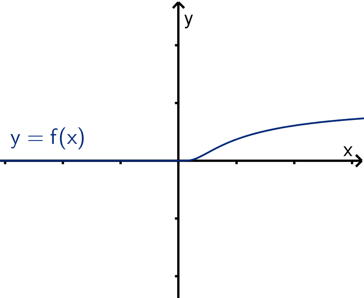
No matter how large n gets, T
n
(x) will not get any closer to f(x) for any x > 0.
How can this happen, given Taylor’s Inequality? The derivatives of f get bigger and bigger. M
grows so fast that the error R
n
(x) gets no smaller even with an (n + 1)! in the denominator of Taylor’s
Inequality.
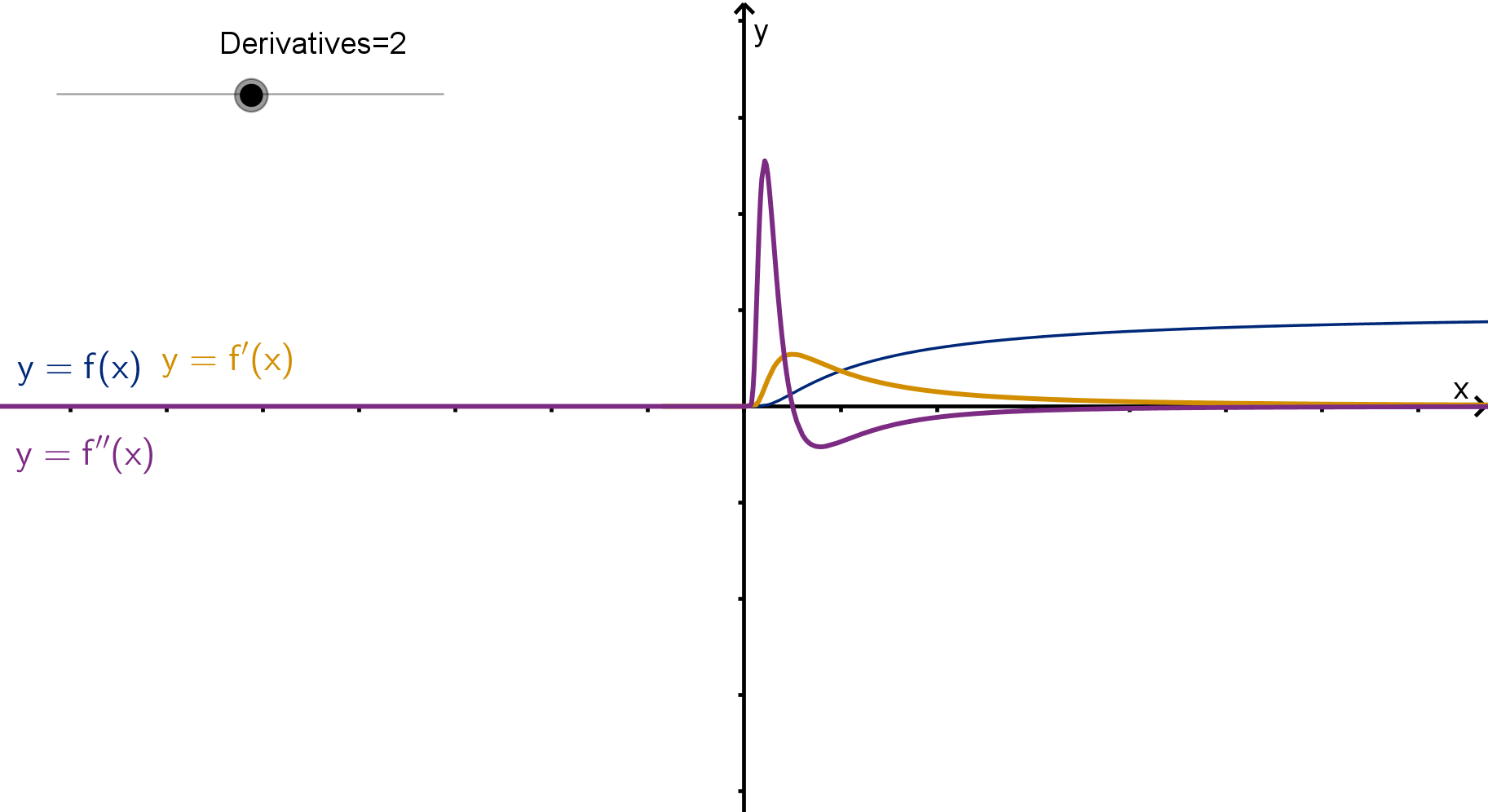
Figure: A function whose derivative bounds grow factorially
Despite examples like this, it turns out that Taylor polynomials often do a good job of approximating
functions. For numerical computations, an approximation is good enough. For more theoretical situ-
ations, we would like to let n go to ∞ so that the error goes to 0 and we can use the polynomial as
an exact replacement of the function. Unfortunately, with infinitely many terms, we no longer have a
polynomial at all. Instead we have an object that we will call a Taylor series. We will develop the tools
to define and work with Taylor series over the course of this chapter.
181
Section 3.1
Exercises
Summary Questions
Q1
Why do we use Taylor polynomials?
Q2
Why is there a denominator of k! in the formula for a Taylor polynomial?
Q3
Explain why we’d always rather center a Taylor polynomial for y = ln x at x = 1.
Q4
What properties make a Taylor polynomial T
n
(x) a better approximation of f(x)?
3.1.1
Q5
Suppose we use the linearization of f (x) =
3
√
x at x = 8 to approximate
3
√
6.
a
What is the relationship between f(x) =
3
√
x and
3
√
6?
b
Suppose L(x) is the the linearization of f (x) at x = 8. Would you expect L(6) to overesti-
mate or underestimate
3
√
6? Explain in a sentence or two.
Q6
Suppose you were locked in a room with only a pencil and paper and asked to compute the first
ten decimal places of the following numbers:
4
17
√
7 e
Which could you compute?
For the ones you can compute, how would you do it?
182
3.1.2
Q7
Is a tangent line a Taylor polynomial?
Q8
Suppose T
4
(x) is the Taylor polynomial for f(x) centered at x = 10. List what information T
4
(x)
and f(x) have in common, being as specific as possible.
Q9
If f (x) is a decreasing function, what can you say about the coefficients of any Taylor polynomial
of f(x)?
Q10
Suppose f(x) has a Taylor polynomial
T
4
(x) = 5 + 3(x − 2) −
1
6
(x − 2)
2
+ 2(x − 2)
4
a
What is f (2)?
b
Is f increasing or decreasing at x = 2?
c
Is f concave up or concave down at x = 2?
3.1.3
Q11
Let f(x) = e
x
.
a
Find the degree 8 Taylor polynomial of y = f(x) centered at x = 0.
b
How could you use this to estimate the value of e?
c
Can you use sigma notation to write a general form for the degree n Taylor polynomial of
y = e
x
?
Q12
Let f(x) = ln x
a
Write the 5th Taylor polynomial of f(x) at x = 1.
b
Use your polynomial to approximate ln 2.
183
Section 3.1
Exercises
Q13
Write the 10th Taylor polynomial for f (x) = cos x centered at x = π.
Q14
Write the 4th Taylor polynomial for f (x) =
1
x
2
centered at x = 5.
3.1.4
Q15
Write each of the following sums in Σ notation.
a
15 − 45 + 105 − 315 + 945
b
24 + 19 + 14 + 9 + 4 − 1 − 6
c
1
8
+
1
18
+
1
50
+
1
72
+
1
98
Q16
Write each of the following sums in Σ notation.
a
11 − 13 + 15 − 17 + 19 − 21 + 23
b
384 + 192 + 96 + 48 + 24 + 12 + 6
c
2
10
+
3
100
+
4
1000
+
5
10000
3.1.5
Q17
Write an expression in Σ notation for the 53rd Taylor polynomial of f (x) = ln x centered at
x = 1
Q18
Write an expression in Σ notation for the 15th Taylor polynomial of f(x) = e
x
centered at x = 0
Q19
Write an expression in Σ notation for the 100th Taylor polynomial of f(x) = cos x centered at
x = 0
Q20
Write an expression in Σ notation for the 71st Taylor polynomial of f (x) =
1
x
2
centered at x = 10
184
3.1.6
Q21
Why don’t we have any theorems for a lower bound for error? Give your answer in a few sentences.
Q22
Suppose you are using Taylor polynomials of f(x) centered at x = 0 to approximate f(−3).
However, for each k, the best bound you can put on f
(k)
(x) on [−3, 0] is
k!
4
k
. Will you be able
to guarantee a good approximation of f(−3) this way? Explain.
Q23
Suppose the fourth derivative of f(x) is f
(4)
(x) = e
x
3
. Suppose we have written T
4
(x), the
degree 4 Taylor polynomial of f(x) centered at x = 1. What can you say about the difference
between T
4
(5) and f(5)? Be specific and justify your answer with a computation. You do not
need to simplify any arithmetic in your calculations.
Q24
Sketch a graph of y = e
x
and several tangent lines. On which part of the graph do the tangent
lines appear to approximate the function better? Does Taylor’s Inequality confirm this observa-
tion? Explain.
3.1.7
Q25
Here is the degree 3 Taylor polynomial of f(x) =
√
x centered at x = 4:
T
3
(x) = 2 +
1
4
(x − 4) −
1
64
(x − 4)
2
+
1
512
(x − 4)
3
a
Which derivative will let you bound the error of this approximation?
b
Can you put a bound on this derivative that holds for all x?
c
Can you put a bound on this derivative that holds for x in the interval [4, 5]?
d
What error bound does this suggest for using T
3
(5) to approximate
√
5?
Q26
Let f(x) =
3
√
x.
a
Write the degree 2 Taylor polynomial of f centered at x = 8.
b
If you wanted to use the Taylor polynomial to approximate
3
√
10, how would you do that?
185
Section 3.1
Exercises
c
What bound could you place on the error in the approximation in
b
?
Q27
Let f(x) = e
x
.
a
Write the degree 5 Taylor polynomial of f centered at 0.
b
How could we use this polynomial to approximate
1
√
e
?
c
Produce an error bound for your approximation in
b
.
Q28
Let f(x) = xe
x
.
a
Compute the Taylor polynomial T
3
(x) for f (x) centered at x = 0.
b
Compute the theoretical error bound for T
3
(2).
c
Explain the difficulties that would arise from this error bound, if your goal is to approximate
f(2) by hand. Can you resolve them?
Q29
Let f(x) = cos 3x
a
Write the degree 4 Taylor polynomial of f centered at x = 0.
b
How would you use that Taylor polynomial to approximate the value of cos
3π
4
?
c
What bound can you place on the error of such an approximation?
Q30
Consider the graph of y = f (x) below.
186
a
Suppose you wanted to produce the second degree Taylor polynomial of f centered at a =
−1. Indicate whether the constant term and each coefficient would be positive or negative.
Provide evidence for your answer.
b
Would T
2
(4) underestimate or overestimate f(4)? Explain.
Synthesis and Extension
Q31
Let f(x) = x
3
− 3x + 5.
a
Write an expression for T
3
(x), the Taylor polynomial centered at x = 2.
b
What can you say about th error R
3
(x) for any x?
c
What relationship does this suggest between f (x) and T
3
(x)?
d
Can you verify this relationship algebraically?
e
Conjecture a general relationship between polynomial functions and certain Taylor polyno-
mials. Can you use Taylor’s inequality to justify your conjecture?
187
Section 3.2
Sequences
Goals:
1 Use notation to describe the terms of an infinite sequence.
2 Calculate the limit of an infinite sequence.
Sequences are the first step in our development of Taylor series. While they appear to have little in
common with polynomials of infinite degree, they are the scaffolding on which such objects are built.
Question 3.2.1
What Is a Sequence?
A sequence is an ordered set of numbers. If this set is infinite, we can most rigorously define it by
giving a general formula for the n
th
term for some index variable n. Here are three different notations
for the same sequence.
1
2
,
2
3
,
3
4
,
4
5
. . .
n
n + 1
∞
n=1
a
n
=
n
n + 1
Example
The first three terms of
n
2
2
n
∞
n=0
are
0
2
2
0
= 0
1
2
2
1
=
1
2
2
2
2
2
= 1
Question 3.2.2
What Is the Limit of a Sequence?
Definition
If we can make the elements of a sequence a
n
arbitrarily close to some number L by considering only n
above a certain number, then we write
lim
n→∞
a
n
= L
and we say the sequence converges to L. If a
n
does not converge to any such L then we say it
diverges.
188
Remarks
The first few or even the first thousand terms of a sequence have no bearing on the limit. We
only care that we can eventually get close to L.
“Arbitrarily close” means any level of closeness than anyone could ask for. Eventually the sequence
must be within
1
100
of L, and
1
1000
and
1
1000000
.
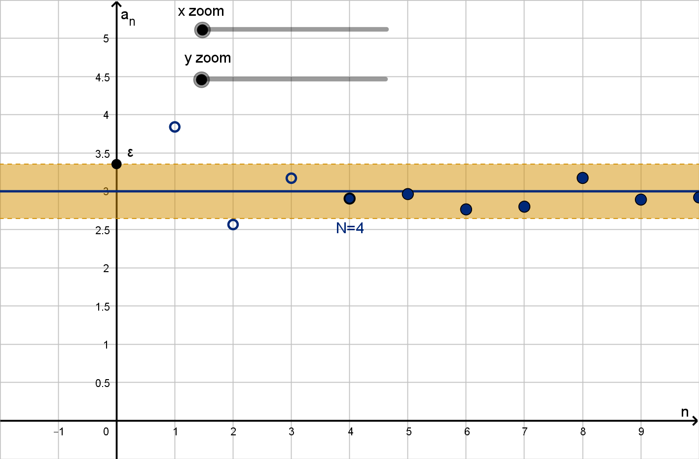
Figure: A sequence converging to L = 3
Example 3.2.3
Computing a Limit
Calculate lim
n→∞
n
n + 1
1
2
,
2
3
,
3
4
,
4
5
. . .
189
Example 3.2.3
Computing a Limit
Solution
Writing the first few terms suggests that this sequence approaches 1. To see that, we can measure the
distance to 1:
1 − a
n
= 1 −
n
n + 1
=
1
n + 1
We can make this smaller than any positive number. For instance to make a
n
within
1
1000
of 1, we can
consider only n > 1000. We conclude lim
n→∞
n
n + 1
= 1
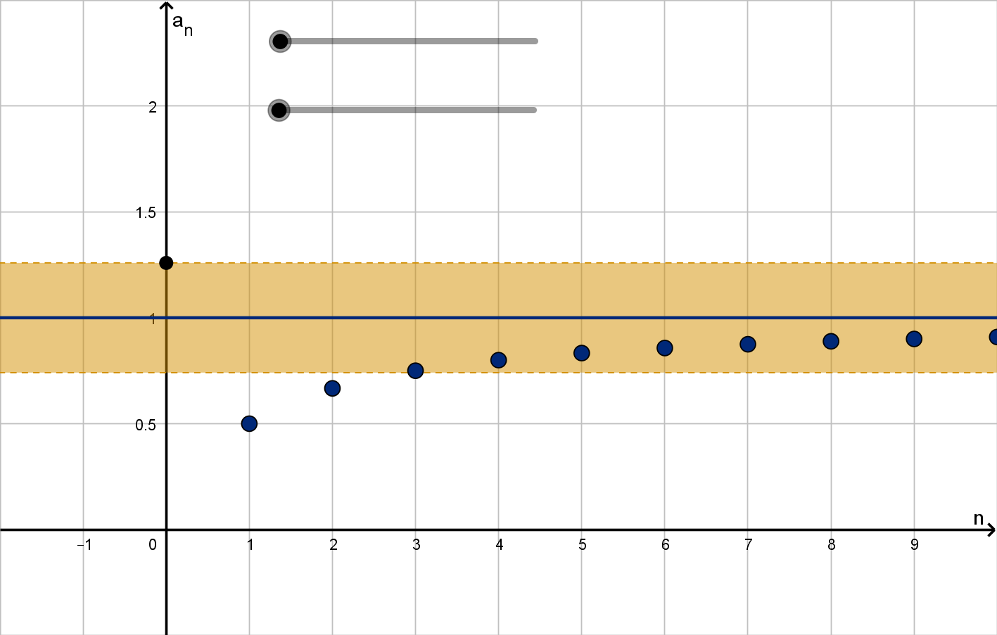
Figure: The sequence
n
n+1
converges to L = 1.
Question 3.2.4
How Are Limits of Sequences and Functions Related?
The definition of lim
n→∞
a
n
should look familiar. The definition of the limit of a function is similar.
In fact, the limit of a f(x) as x → ∞ has a nearly identical construction, except that n must be an
integer, while x can be any real number. The following theorem lets us use that connection to evaluate
limits.
190
Theorem
Suppose for a sequence a
n
, there is a function f (x) such that f(n) = a
n
for all n (or at least all n
sufficiently large). If
lim
x→∞
f(x) = L
we can conclude that
lim
n→∞
a
n
= L.
Example 3.2.5
Sequence Limits Using Functions
Find limits of the following sequences:
a
lim
n→∞
2n
n + 3
b
lim
n→∞
1
n
3
c
lim
n→∞
e
−n
d
lim
n→∞
n
2
e
n
e
lim
n→∞
(−1)
n
Solution
We will use x to denote a real number variable and n to denote natural numbers.
a
lim
x→∞
2x
x + 3
= 2, so lim
n→∞
2n
n + 3
= 2.
b
lim
x→∞
1
x
3
= 0, so lim
n→∞
1
n
3
= 0.
c
lim
x→∞
e
−x
= 0 so lim
n→∞
e
−n
= 0.
191
Example 3.2.5
Sequence Limits Using Functions
d
lim
x→∞
x
2
e
x
can be evaluated with L’hˆopital’s rule.
lim
x→∞
x
2
e
x
= lim
x→∞
2x
e
x
∞
∞
form, L’hˆopital’s again
= lim
x→∞
2
e
x
= 0so lim
n→∞
n
2
e
n
= 0
e
f(x) = (−1)
x
is not well defined for real numbers so we can’t use its limit. Instead examine the
sequence directly. The sequence has the form
−1, 1, −1, 1, −1, 1, −1, 1, . . .
This does not approach arbitrarily close to any number. No matter how many early terms we
disregard, there will always be terms remaining that are not close to 1, or not close to −1 or not
close to any other number. Thus a
n
= (−1)
n
diverges.
The following limit laws for sequences should look familiar. They mirror the laws for limits of
functions.
Theorem [Limit Laws]
If lim
n→∞
a
n
= K and lim
n→∞
b
n
= L then the following sequences converge with the following limits:
lim
n→∞
(a
n
+ b
n
) = K + L
lim
n→∞
(a
n
− b
n
) = K − L
lim
n→∞
(a
n
b
n
) = KL
If L = 0, then lim
n→∞
a
n
b
n
=
K
L
For any constant c, lim
n→∞
ca
n
= cK
192
Synthesis 3.2.6
Indeterminate Forms with Factorials
We will encounter sequences of the form a
n
=
b
n
c
n
. If b
n
or c
n
both go to 0 or ±∞, then any attempt
to use
lim
n→∞
a
n
= lim
x→∞
f(x)
would require l’Hˆopital’s rule.
Dominance
We say f (x) dominates g(x) if lim
x→∞
f(x)
g(x)
= ±∞. We write
f(x) >> g(x)
Even if you include a constant multiple or add multiple functions together, the dominant function
will outgrow any combination of dominated ones. We have already established an order of dominance
using l’Hˆopital’s rule:
exponential
(larger base>>smaller base)
>>
polynomial
(larger degree>>smaller)
>>
root
(smaller power>>larger)
>>
logarithm
(smaller base>>larger)
But n! is not a differentiable function. We cannot analyze it using l’Hˆopital’s rule. Where does it fit
in the domincance pecking order?
Theorem
As n → ∞, n! will eventually dominate any exponential function (and thus any polynomial, root or
logarithm).
We will not provide a formal proof, but here is a useful thought experiment. Suppose we compare
n! to 63
n
. At first 63
n
grows faster, multiplying by 63 every time we increase n. However, when n is
greater than 63, n! is multiplying by a higher number. When n reaches one billion, 63
n
increases by a
factor of 63 every step, while n! increases by a factor of 1, 000, 000, 000. By this point n! is much larger
and growing much faster.
193
Section 3.2
Exercises
Summary Questions
Q1
Why do we use n instead of x as an index for a sequence?
Q2
Describe three different ways of denoting a sequence.
Q3
When is the limit of a sequence equal to the limit of a function?
Q4
If a
n
= b
n
+ 1000 for 1 ≤ n ≤ 2000000, what does that tell us about the limits lim
n→∞
a
n
and
lim
n→∞
b
n
?
3.2.1
Q5
Find a general expression for a
n
, the n
th
term of the following sequences. Use this to write the
sequences using both other types of notation.
a
{2, 5, 10, 17, 26, 37, 50, . . .}
b
3
2
, −
3
4
,
3
8
, −
3
16
,
3
32
, . . .
c
1
2
,
1
6
,
1
12
,
1
20
,
1
30
, . . .
Q6
What is the fourth term in the sequence {n
3
− 5n}
∞
n=3
?
194
3.2.2
Q7
Show using the definition of the limit of a sequence that lim
n→∞
sin n
n
2
= 0.
Q8
Show using the definition of the limit of a sequence that lim
n→∞
2
n
− 1
2
n
= 1.
Q9
A sequence is increasing if every term is larger than the previous term. Must an increasing
sequence always diverge? Explain.
Q10
A sequence is alternating if its terms alternate between positive and negative values. Is it possible
that the limit of an alternating sequence exists? What would its value have to be?
3.2.3
Q11
Consider the sequence a
n
= 2
n
.
a
What function could we write such that f(n) = a
n
.
b
Does lim
x→∞
f(x) converge?
c
Does the theorem equating limits of functions and sequences apply to this function?
d
Can we argue that lim
n→∞
2
n
diverges anyway?
Q12
Consider the sequence a
n
= n sin(πn)
a
What is lim
x→∞
x sin(πx)?
b
Compute the first few values a
1
, a
2
, a
3
, and a
4
.
c
What is lim
n→∞
n sin(πn)?
d
Does this contradict one of our theorems? Explain.
195
Section 3.2
Exercises
3.2.4
Q13
Compute lim
n→∞
log n
3n
.
Q14
Compute lim
n→∞
n
2
n
.
Q15
Compute lim
n→∞
n
3
+ 3
4n
3
− 9
.
Q16
Compute lim
n→∞
sin n
log n
.
Q17
Compute lim
n→∞
e
n
√
n
.
Q18
Compute lim
n→∞
tan
−1
n.
3.2.5
Q19
Compute lim
n→∞
n!
5
n
.
Q20
Compute lim
n→∞
n
4
+ 3n + 1
n!
.
Q21
Does n
n
grow faster or slower than n!? Explain.
Q22
Yuran knows that lim
n→∞
n!
5
n
= ∞ because n! growns faster than a
n
. However, he thinks he can
make the denominator grown faster than the numerator if he uses a product like
n!
5
n
6
n
or
n!
5
n
6
n
7
n
.
Will he eventually obtain a non-infinite limit by this method? Explain how you know.
196
Synthesis & Extension
Q23
Suppose we have a sequence a
n
=
(
f(n) if n ≤ 342
g(n) if n > 342
. Which of the following could help us
evaluate lim
n→∞
a
n
?
lim
x→∞
f(x)
lim
x→∞
g(x)
Q24
Let T
n
(x) be the nth Taylor polynomial of f(x) = ln x centered at x = 1.
a
Write an expression for T
n
(x) using Σ notation.
b
Write an expression for the error bound of T
n
(x) for some x between 0 and 1.
c
For what values of x will the error bound shrink to 0 as n goes to ∞?
197
Section 3.3
Series
Goals:
1 Identify partial sums of a series.
2 Recognize harmonic and alternating harmonic series.
3 Apply the divergence test.
4 Evaluate geometric series.
5 Apply the ratio test.
The first step in understanding a Taylor polynomial of infinite degree is understanding how to add
up infinitely many of anything. This proposition is mechanically absurd. Addition is an operation for
two numbers at a time. Adding three or four numbers requires us to add two or three times. Adding
infinitely many requires us to add infinitely many times, something no one has time to do.
Yet there are some intuitive exercises we could perform. Suppose we lay a length of
1
2
m next to
1
4
m
next to
1
8
m. If we continued indefinitely, we could imagine these lengths extending an entire meter.
Figure: One meter expressed as a sum of infinitely many smaller lengths
What reasoning could we use to make this exercise rigorous? How could we add up lengths or
numbers where the pattern is not so intuitive? The formal object that does this is called a series. A
series is the first step on our way to push the Taylor polynomial to infinite degree. It is also the most
general. While we are concerned with one specific (and very useful) type of series, there are other
applications worth exploring as well.
Question 3.3.1
What Is a Series?
You have been encountering series since you first learned about decimals. You likely have not seen
a rigorous description of what they mean.
0.33333333 . . . 3.1415926...
We can write
0.3333 . . . =
3
10
+
3
100
+
3
1000
+
3
10000
+ ···
or
3.1415 . . . = 3 +
1
10
+
4
100
+
1
1000
+
5
10000
+ ···
You may have an intuitive sense of what these quantities are, but what does it mean to add up
infinitely many numbers?
198
Definition
A series is a sum of the form
∞
X
k=1
a
k
where a
k
is an infinite sequence. If it is more convenient, we can
give k a different initial value. If the context is clear, we can write
X
a
k
as a shorthand.
Example
0.33333 . . . =
∞
X
k=1
3
10
k
The harmonic series is
∞
X
k=1
1
k
This tells us what a series is but not how to evaluate it. How do we know that, for example
0.333 . . . =
1
3
?
We evaluate a series by associating it with a sequence of partial sums.
Definition
The n
th
partial sum of the series
∞
X
k=1
a
k
is
s
n
= a
1
+ a
2
+ a
3
+ ··· + a
n
A series
∞
X
k=1
a
k
converges to L if
lim
n→∞
s
n
= L.
A series that does not converge to any L diverges.
Vocabulary Note
Do not confuse a sequence with a series. One is a list of numbers. The other is the sum of a list of
numbers.
199
Example 3.3.2
Computing Partial Sums
Consider
∞
X
k=1
3
10
k
.
a
Compute the first few partial sums s
1
, s
2
, s
3
of this series.
b
Compute lim
n→∞
s
n
Solution
a
s
1
=
3
10
s
2
=
3
10
+
3
100
=
33
100
s
3
=
3
10
+
3
100
+
3
1000
=
333
1000
s
4
=
3
10
+
3
100
+
3
1000
+
3
10000
=
3333
10000
b
In order to use our usual methods of limits, we would need an algebraic expression for s
n
. It isn’t
immediately clear how to produce one. Given our knowledge of decimals, we expect the answer
to be
1
3
. We will use this as a hint. We expect
1
3
− s
n
to approach 0.
1
3
− s
1
=
1
30
1
3
− s
2
=
1
300
1
3
− s
3
=
1
3000
1
3
− s
4
=
1
30000
extrapolating suggests
1
3
− s
n
=
1
3(10)
n
Assuming this pattern holds, we have
lim
n→∞
1
3
− s
n
= lim
n→∞
1
3(10)
n
= 0
and we conclude that
∞
X
k=1
3
10
k
=
1
3
.
200
Main Idea
Often, we can show that
∞
X
k=1
a
k
= L by computing L − s
n
and seeing that it converges to 0.
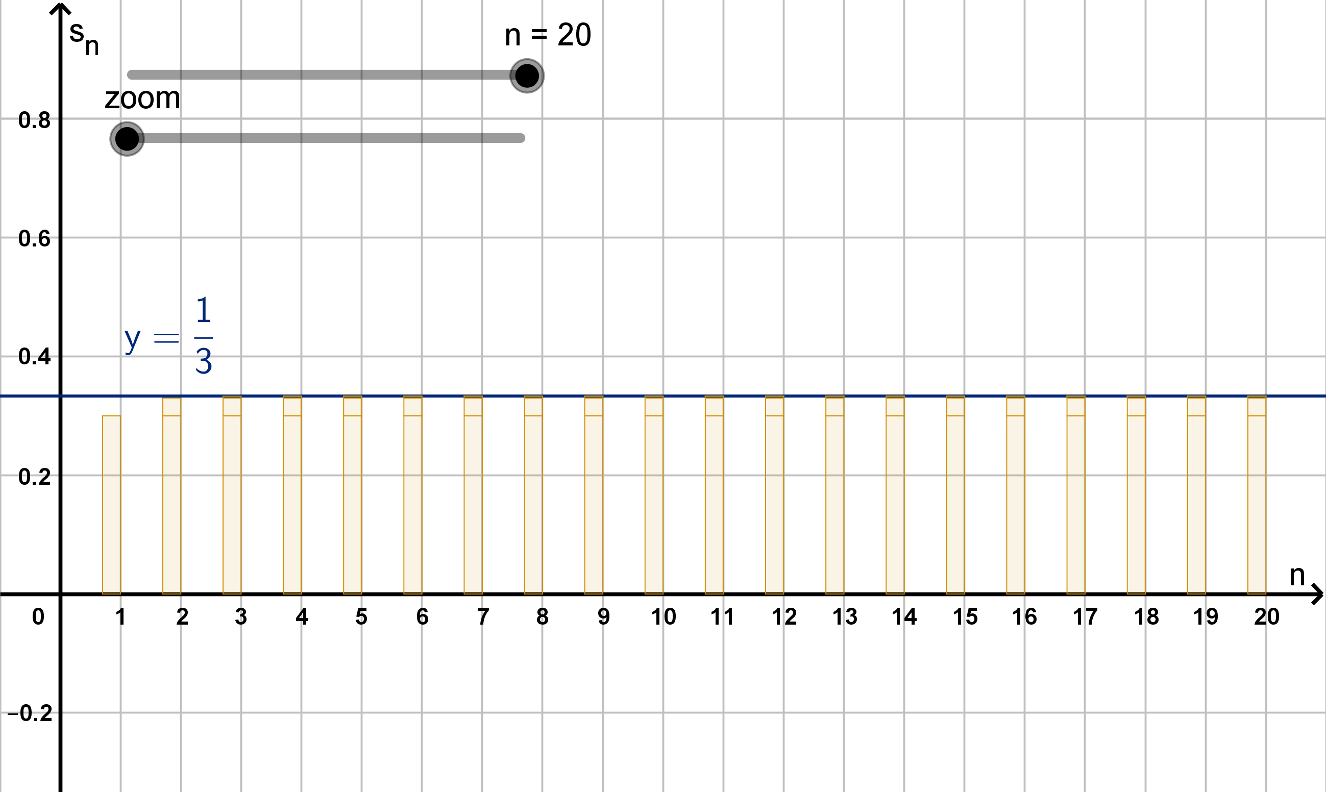
Figure: The partial sums s
n
converging to L =
1
3
Example 3.3.3
The Harmonic Series
We have seen examples of series in which the terms approach 0 as k → ∞. These have allowed us
to add infinitely many terms and obtain a finite sum. Does this always work? No. A series can have its
terms approach 0, and yet the partial sums go to ∞. The most famous example of this is the harmonic
series:
∞
X
k=1
1
k
. Rather than computing the partial sums directly (which would be a lot of computation)
we will compare the partial sums to an expression that is easier to calculate. We will replace each term
by a fraction with a power of 2 in the denominator. Here’s what we’ll do with s
8
.
s
8
=
1
1
+
1
2
+
1
3
+
1
4
+
1
5
+
1
6
+
1
7
+
1
8
>
1
1
+
1
2
+
1
4
+
1
4
| {z }
1
2
+
1
8
+
1
8
+
1
8
+
1
8
| {z }
1
2
=1 +
1
2
+
1
2
+
1
2
Since we replaced each term with something smaller and obtained a sum of
5
2
, we can conclude that
s
8
>
5
2
. Continuing this pattern, the terms
1
9
to
1
16
sum to more than
1
2
so s
16
>
6
2
. In general we can
201
Example 3.3.3
The Harmonic Series
make s
n
bigger than any integer c by setting n = 2
m
where
1 +
1
2
m > c.
This tells us that the harmonic series diverges.
Question 3.3.4
What Is a Geometric Series?
The two series so far that we have been able to evaluate belonged to a larger family. These are the
geometric series.
Definition
A geometric series is a series of the form
∞
X
k=1
ar
k−1
.
a is the initial term. r is the common ratio between terms.
Example
∞
X
k=1
1
2
k−1
= 1 +
1
2
+
1
4
+
1
8
+ ···
∞
X
k=1
3
10
1
10
k−1
=
3
10
+
3
100
+
3
1000
+ ··· =
1
3
Unlike many other series, geometric series are simple enough that we can write a formula for their
sum. We can get a convenient expression for s
n
by performing a cute algebra trick. We’ll multiply s
n
by r and subtract rs
n
from s
n
. Most of the terms cancel and we obtain an equation that we can solve
for s
n
.
s
n
= a + ar + ar
2
+ ··· + ar
n−1
−rs
n
= −ar − ar
2
− ar
3
− ··· − ar
n
(1 − r)s
n
= a − ar
n
s
n
=
a(1 − r
n
)
1 − r
The last step requires that 1 − r = 0, since we cannot divide by 0. As long as r = 1, we can evaluate
the series by taking a limit.
∞
X
k=1
ar
k−1
= lim
n→∞
a(1 − r
n
)
1 − r
202
To evaluate this limit, we need to understand the behavior of r
n
as n → ∞
If −1 < r < 1 then higher powers of r get smaller and smaller and r
n
→ 0.
If r > 1 then higher powers of r get larger and larger and r
n
→ ∞.
If r < −1 then higher powers of r get larger but alternate signs. lim
n→∞
r
n
does not exist.
If r = 1 then the series is a + a + a+ a + a + ···, then s
n
= an which diverges to ±∞, depending
on the sign of a.
If r = −1 then the series is a − a + a − a + a − ···, then s
n
alternates between a and 0. This
sequence does not converge.
We can apply the above to completely solve the problem of evaluating a geometric series. Our result is
the following theorem:
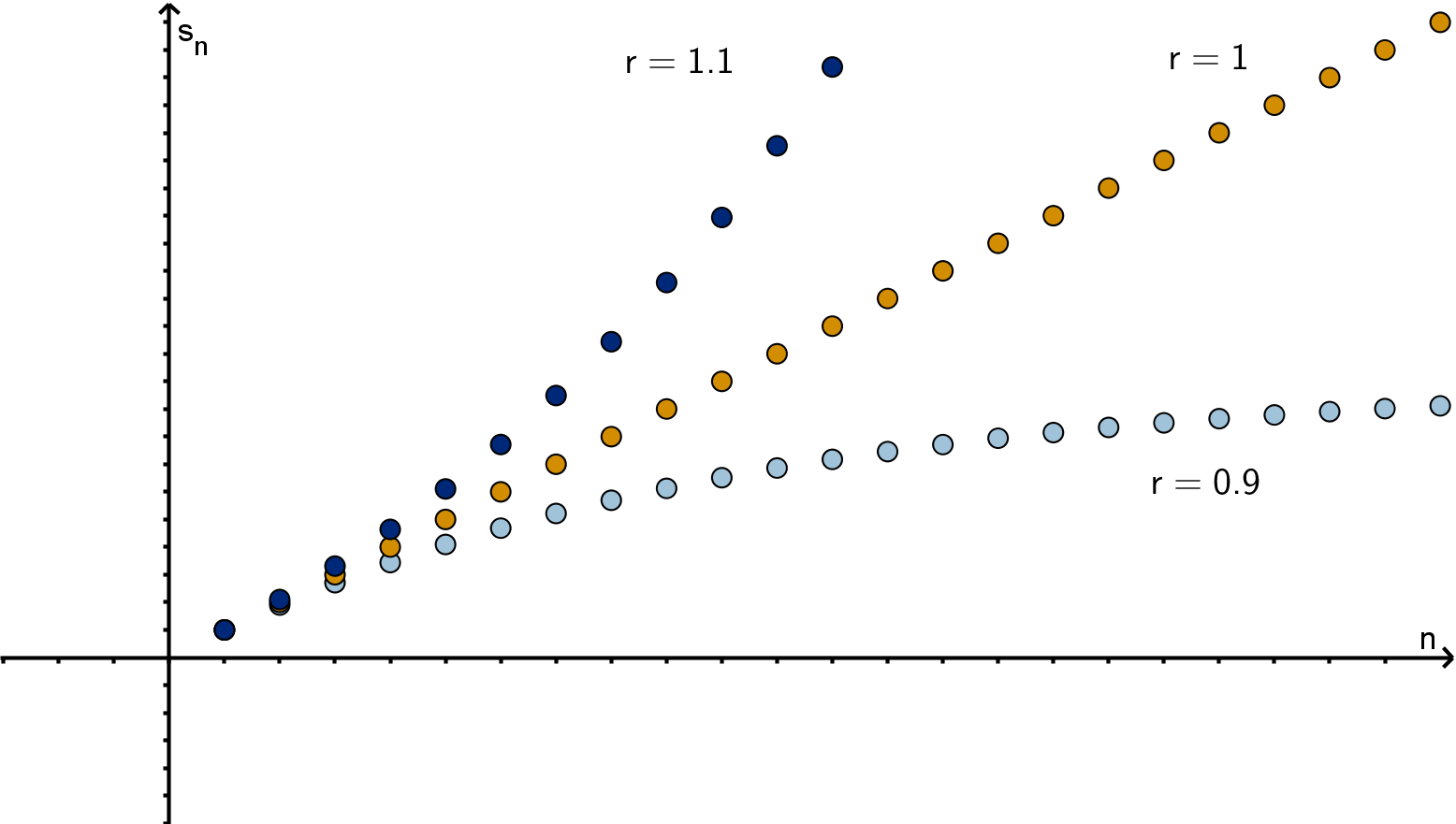
Figure: The partial sums of
P
ar
k−1
for various r
Theorem
Geometric series have the following partial sums
s
n
=
n
X
k=1
ar
k−1
=
a(1 − r
n
)
1 − r
if r = 1
an if r = 1
These converge to
a
1 − r
when |r| < 1 and diverge when |r| ≥ 1.
203
Example 3.3.5
Evaluating Geometric Series
Identify a and r in the following geometric series. Then evaluate the series.
a
2
3
+
4
15
+
8
75
+ ···
b
∞
X
n=2
3
n
c
0.999999 . . .
Solution
a
a is the initial term, which is
2
3
. The common ratio is the ratio between any two terms.
4/15
2/3
=
2
5
.
Since |r| < 1, the sum of the series is
∞
X
k=1
2
3
2
5
k−1
=
2
3
1 −
2
5
=
2
3
3
5
=
10
9
b
The initial term of this series is 9. The common ratio is 3. Since |3| ≥ 1,
∞
X
n=2
3
n
diverges.
c
0.999999 . . . =
9
10
+
9
100
+
9
1000
+ ···. This has an initial term of
9
10
and a common ratio of
1
10
.
|r| < 1 so
0.999999 . . . =
9
10
1 −
1
10
=
9
10
9
10
= 1
204
Question 3.3.6
What Does the Size of a
k
Tell Us About
P
a
k
?
The discussion of the geometric series suggests that certain properties of a series make convergence
impossible. Specifically, in the cases in which the terms were not shrinking to 0, the partial sums were
growing without bound or oscillating. This intuition can be formalized in the following theorem, which
applies to more than just geometric series.
Theorem [The Divergence Test]
Let a
k
be a sequence. If lim
k→∞
a
k
= 0, then the series
∞
X
k=1
a
k
diverges.
Remark
The divergence test does not tell us anything, if lim
k→∞
a
k
= 0. The series might converge, and it might
not. In this case we say the test is inconclusive.
Example 3.3.7
Applying the Divergence Test
What does the divergence test tell us about each of the following series?
a
∞
X
k=2
3
k
b
∞
X
k=2
1
k
c
∞
X
k=2
k
2
− 1
3k
2
+ 7
d
∞
X
k=2
k
2
e
k
205
Example 3.3.7
Applying the Divergence Test
Solution
a
The sequence is a
k
= 3
k
. lim
k→∞
3
k
= ∞. This limit is not 0, so by the divergence test, the series
diverges.
b
The sequence is a
k
=
1
k
. lim
k→∞
1
k
= 0. The divergence test is inconclusive. It cannot tell us
whether this series diverges or converges. By our earlier work, we happen to know this series
diverges.
c
The sequence is a
k
=
k
2
−1
3k
2
+7
. lim
k→∞
k
2
− 1
3k
2
+ 7
=
1
3
. This limit is not 0, so by the divergence test,
the series diverges.
d
The sequence is a
k
=
k
2
e
k
. We need L’Hˆoptial’s rule to evaluate the limit.
lim
k→∞
k
2
e
k
= lim
k→∞
2k
e
k
still
∞
∞
form
= lim
k→∞
2
e
k
= 0
The divergence test is inconclusive. It cannot tell us whether this series diverges or converges. It
turns out that this series converges, but we do not have a method to verify that yet.
Question 3.3.8
What Is the Ratio Test?
So far we have two tests to determine the convergence of a series. One test is very specific, applying
only to geometric series. The other is very imprecise. The divergence test is often inconclusive. It
does not help us to evaluate a series at all, only recognizing some series that diverge. Unfortunately,
these shortcoming are typical of series tests. A rigorous study of infinite series requires learning almost a
dozen tests. On a randomly chosen series, most of these tests will be inconclusive, and none of them will
give a numerical value, even if the series happens to converge. Because we are interested in extending
Taylor polynomials to have infinitely many terms, some of these tests are much more useful than others.
The most useful is the ratio test, though it is still no help in evaluating a series and is still sometimes
inconclusive.
In the case of a geometric series,
P
ar
k−1
, the common ratio between terms determines whether this
series grows out of control, or whether the terms shrink quickly enough that the partial sums converge.
Even when a series is not geometric, we can attempt to apply similar reasoning to determine whether it
converges. A non-geometric series does not have a constant ratio. The ratio between successive terms
will change as we progress through them. We will instead compute the limit of these ratios.
206
Theorem [The Ratio Test]
If lim
k→∞
a
k+1
a
k
= L < 1, then
X
a
k
converges absolutely.
If lim
k→∞
a
k+1
a
k
= L > 1 or is infinite, then
X
a
k
is divergent.
If lim
k→∞
a
k+1
a
k
= 1, then the ratio test is inconclusive.
Remark
Converges absolutely is a term for series with both positive and negative terms. It means the series
would converge, even if the signs of all the terms were all positive. The alternative is conditional
convergence, meaning the series’s convergence may require the positive and negative terms partially
canceling each other out.
Example
The series
1 −
1
2
+
1
3
−
1
4
+
1
5
− ···
converges (we won’t prove this). If we made all the terms positive, it would be the harmonic series,
which diverges. This series converges conditionally, not absolutely.
Absolute versus conditional convergence can be interesting to play with. You may see references to
it in other math books, but we won’t have any further use for it.
Example 3.3.9
Applying the Ratio Test
a
Does
∞
X
k=1
(−1)
k−1
k!
converge or diverge?
b
Does
∞
X
k=1
2
k
k
2
converge or diverge?
c
Does
∞
X
k=1
k converge or diverge?
207
Example 3.3.9
Applying the Ratio Test
Solution
a
First we will compute and simplify the ratio. Then we will take its limit and draw a conclusion.
a
k+1
a
k
=
(−1)
k
(k+1)!
(−1)
k−1
k!
=
(−1)
k
k!
(−1)
k−1
(k + 1)!
=
(−1)
k
(1)(2)(3) ···(k)
(−1)
k−1
(1)(2)(3) ···(k)(k + 1)
(expand the factorials)
=
(−1)
k
(−1)
k−1
(k + 1)
(cancel the matching factors)
=
−1
k + 1
(cancel k − 1 powers of − 1)
=
1
k + 1
(absolute value of a negative number is its negatve)
Now we take the limit
lim
k→∞
1
k + 1
= 0
0 < 1 so by the ratio test,
∞
X
k=1
(−1)
k−1
k!
converges.
b
We will apply the ratio test. First we compute the ratio, and then we take a limit.
a
k+1
a
k
=
2
k+1
(k+1)
2
2
k
k
2
=
2
k+1
k
2
2
k
(k
2
+ 2k + 1)
=
2k
2
k
2
+ 2k + 1
(cancel the 2s)
=
2k
2
k
2
+ 2k + 1
lim
k→∞
2k
2
k
2
+ 2k + 1
= 2
2 > 1 so by the ratio test, this series diverges.
208
c
We will apply the ratio test. First we compute the ratio, and then we take a limit.
a
k+1
a
k
=
k + 1
k
=
k + 1
k
lim
k→∞
k + 1
k
= 1
Here the ratio test is inconclusive. It cannot tell whether this series converges or diverges. However,
we can probably figure this out another way. The terms of this series are increasing, which means
the partial sums will grow faster and faster. This was the reasoning behind the divergence test.
lim
k→∞
k = ∞
Since lim
k→∞
k = 0, the divergence test concludes that the series diverges.
Main Ideas
When applying the ratio test, be sure to replace every k with k + 1 for the a
k+1
term.
Familiarize yourself with the algebra rules that allow you to simplify ratios of exponentials and
factorials.
Example 3.3.10
A Strategy for Series Tests
209
Example 3.3.10
A Strategy for Series Tests
Strategy
Given the three ways we have to test for divergence and convergence and the relative ease of applying
each, here is a reasonable approach to testing a series.
Check lim
n→∞
a
n
by dominance
Compute
a
n+1
a
n
Compute lim
n→∞
a
n+1
a
n
P
a
n
converges
P
a
n
diverges
Inconclusive, look up another test
not zero
zero
hard to tell
constant |r| ≥ 1 constant |r| < 1
not constant
< 1> 1
= 1
hard to tell
Let’s apply our strategy to see what we can tell about
∞
X
n=1
1
n
2
.
Solution
First we’ll check that the terms go to zero. If they don’t we quickly classify this as a divergent series.
lim
n→∞
1
n
2
= 0
They do, so we need another check. Now we’ll compute the ratio between terms.
a
n+1
a
n
=
1
(n+1)
2
1
n
2
=
n
2
n
2
+ 2n + 1
This is not a constant; it depends on n. Thus a
n
is not a geometric series. We’ll try the ratio test.
lim
n→∞
a
n+1
a
n
= lim
n→∞
n
2
n
2
+ 2n + 1
= lim
n→∞
n
2
n
2
+ 2n + 1
= 1
This means that the ratio test is inconclusive. We do not know whether this series converges or diverges.
We have exhausted all our tests. If we want the answer, we need to look up another test.
210
Section 3.3
Exercises
Summary Questions
Q1
What is the difference between a sequence and a series?
Q2
How do we evaluate a series?
Q3
What is a geometric series. How do we evaluate one?
Q4
What does it mean to say that a series test is inconclusive?
Q5
How do each of the following factors behave in the ratio
a
k+1
a
k
?
a
k
p
(p a constant)
b
c
k
(c a constant)
c
k!
Q6
How would the ratio test apply to a geometric series
X
ar
k−1
?
3.3.1
Q7
Give a more common name for each of the following series.
a
2 +
7
10
+
1
100
+
8
1000
+
2
10000
+
8
100000
+ ···
b
6
10
+
6
100
+
6
1000
+
6
10000
+ ···
Q8
Use a calculator to get a decimal approximation of
25
33
and write it as a series of fractions with
powers of 10 as denominators.
211
Section 3.3
Exercises
3.3.2
Q9
Consider the series
∞
X
k=1
1
k(k + 1)
a
Compute the first four elements in the series.
b
Compute the partial sums: s
1
, s
2
, s
3
, s
4
.
c
What do the partial sums appear to be converging to?
d
Can you use algebra to generalize your answer to
2
to s
n
?
Q10
Compute the first 3 partial sums of
∞
X
k=1
k + 1
k
2
. Don’t simplify the arithmetic.
Q11
Compute the first four partial sums of
∞
X
k=1
(−1)
k
. What do you think this suggests about the sum
of the series?
Q12
Compute the first five partial sums of
∞
X
k=0
1
(−2)
k
. Use them to make a prediction about the value
of the series.
3.3.3
Q13
Give an example of an n such that you know the nth partial sum of the harmonic series is greater
than 20.
Q14
Modify our argument for the harmonic series to show that
∞
X
k=0
1
√
k
diverges?
212
3.3.4
Q15
Is
1
2
+
1
4
+
1
6
+
1
8
+ ··· a geometric series? How can you tell?
Q16
Is 1 + 4 + 9 + 16 + 25 + ··· a geometric series? How can you tell?
Q17
The first two terms of a geometric series are 5 and 7.5. What is the third term?
Q18
The fifth term of a geometric series is 17. The eigth term is 51. What is the sixth term?
3.3.5
Q19
Evaluate
∞
X
k=0
5(0.3)
k
Q20
Evaluate
∞
X
k=0
1
4
4
3
k
.
Q21
Evaluate
∞
X
j=3
15
5
j
.
Q22
Evaluate
∞
X
k=1
0.8
k
.
Q23
Evaluate
∞
X
k=4
3
k
2
k
(18)
.
Q24
Evaluate
∞
X
k=1
37
100
k
. What decimal does this represent?
Q25
For what values of z does
∞
X
k=0
3
k
z
k
converge?
Q26
For what values of p does
∞
X
k=3
12p
2k
16
k
converge?
213
Section 3.3
Exercises
3.3.6
Q27
If a
k
>
1
100
for all k, then what can you say about the value of s
n
=
n
X
k=1
a
k
?
Q28
If lim
k→∞
a
k
=
1
100
, use the definition of a limit and the reasoning in the previous exercise to
show that
∞
X
k=1
a
n
diverges.
3.3.7
Q29
What does the divergence test say about
∞
X
k=1
1
k
3
?
Q30
What does the divergence test say about
∞
X
k=1
k
2
+ 1
5k
2
+ 3k
?
Q31
What does the divergence test say about
∞
X
k=2
ln k?
Q32
What does the divergence test say about
∞
X
k=2
1
ln k
?
3.3.8
Q33
Will the divergence test detect every series that “fails” the ratio test (L > 1)? Explain.
Q34
If lim
n→∞
an + 1
a
n
does not exist, the ratio test is inconclusive. Give examples of two series where
this limit does not exist, one series that diverges and one that converges.
214
3.3.9
Q35
Apply the ratio test to
∞
X
k=1
k!
4
k
. What can you conclude?
Q36
Apply the ratio test to
∞
X
k=1
k5
k
(k + 1)
2
. What can you conclude?
Q37
Apply the ratio test to
∞
X
k=1
(−1)
k−1
k
2
. What can you conclude?
Q38
Apply the ratio test to
∞
X
k=1
(−8)
k
k
2
5
k
. What can you conclude?
Q39
Apply the ratio test to
∞
X
k=1
k
2
4
k
. What can you conclude?
Q40
Apply the ratio test to
∞
X
k=3
k!
5k
3
+ 4k − 2
. What can you conclude?
Q41
Apply the ratio test to
∞
X
k=1
√
k + 1
k
2
What can you conclude?
Q42
Apply the ratio test to
∞
X
k=1
√
ke
−k
What can you conclude?
3.3.10
Q43
Use one of the tests from this section to deterine whether
P
∞
k=1
k+1
k
converges.
Q44
Use one of the tests from this section to deterine whether
P
∞
k=1
3(4
k
)
7
k
converges.
Q45
Use one of the tests from this section to deterine whether
P
∞
k=1
ke
k
4
k+1
converges.
Q46
Use one of the tests from this section to deterine whether
P
∞
k=1
7k9
k
k3
2k+1
converges.
215
Section 3.3
Exercises
Synthesis & Extension
Q47
In a paragraph or two, explain: How is evaluating an improper integral similar to evaluating an
infinite series. How are they different?
Q48
Suppose we have a sequence a
n
such that lim
n→∞
a
n
= 0 and
∞
X
n=1
a
n
= 437. Suppose we then
increase the values of the first five terms of a
n
by 10, 000 each.
a
Explain how this will affect the value of lim
n→∞
a
n
.
b
Explain how this will affect the value of
∞
X
n=1
a
n
.
Q49
Suppose we wanted to approximate
R
∞
0
1
e
x
dx by rectangles of length ∆x = 1, with heights
measured at the left endpoints.
a
What are the areas of the first 5 rectangles, starting from x = 0?
b
How many rectangles will you need in total?
c
Express the sum of the areas of these rectangles as a series.
d
Does this series converge? To what value?
e
Does your series over- or underestimate the true value of the integral?
Q50
Suppose we wanted to approximate
R
∞
1
1
x
2
dx by rectangles of length ∆x = 1, with heights
measured at the right endpoints.
a
What are the areas of the first 5 rectangles, starting from x = 1?
b
Express the sum of the areas of all the the rectangles you’ll need as a series.
c
Does your series over- or underestimate the true value of the integral?
d
What is the true value of the integral? What does this suggest about whether your series
converges or diverges?
Q51
Suppose that a discrete random variable X has distribution function
f
X
(x) =
(
1
2
x
if x is a positive integer
0 otherwise
216
a
Verify that f
X
(x) is a valid probability distribution function.
b
Compute P (X > 4).
c
Compute E[X] (this is difficult).
Q52
Suppose that a discrete random variable X has distribution function
f
X
(x) =
(
1
x
−
1
x+1
if x is a positive integer
0 otherwise
a
Verify that f
X
(x) is a valid probability distribution function.
b
Compute P (3 ≤ X ≤ 5).
c
Explain why you can’t compute E[X].
217
Section 3.4
Power Series
Goals:
1 Use series tests to determine for what values of x a power series converges.
2 Identify the radius of convergence of a power series.
3 Recognize functions that can be rewritten as a power series.
The infinite degree polynomials we seek to define are series. The tools we’ve developed so far
provide the foundation for understanding the objects we want to construct, but there is more to do. A
polynomial also contains a variable. In this section we deal with the ramifications of including a variable
in an infinite series.
Question 3.4.1
What Is a Power Series?
So far we have studied infinite series of numbers. If instead of just numbers, our terms include
variables, then we’ve created a function. Plugging in different values for the variable gives us a different
series of numbers.
Example
The expression
1 + x + x
2
+ x
3
+ ···
becomes
1 + 2 + 4 + 8 + ···
when we evaluate it at x = 2. It becomes
1 −
1
3
+
1
9
−
1
27
+ ···
when we evaluate it at x = −
1
3
.
Definition
An infinite series of the form
∞
X
k=0
c
k
(x − a)
k
is called a power series centered at a.
It is a function of x whose domain is all values of x that make the series converge.
For the purposes of this definition, we define x
0
= 1 even when x = 0.
218
Example 3.4.2
A Geometric Series as a Power Series
Use the geometric series formula to write f (x) =
1
1 − x
as a power series and find its domain.
Solution
1
1 − x
is the sum of a geometric series. In this case, the initial term a = 1 and the common ratio r is
x. If we write out the first few terms we obtain 1 + x + x
2
+ x
3
+ ···. We see this is a power series
centered at 0. The coefficients c
k
are all equal to 1. We could write it as
P
∞
k=0
x
k
.
The domain of a power series is the values of x that make it converge. We know that this geometric
series converges if and only if the common ratio x has absolute value less than 1. Those values of x,
the open interval (−1, 1), are the domain of f.
Example 3.4.3
The Domain of a Power Series
What is the domain of
∞
X
k=1
k
2
4
k
(x − 5)
k
?
Solution
The domain is the set of x values that make the series converge. The ratio test will be helpful here.
The ratio between terms is
a
k+1
a
k
=
(k+1)
2
4
k+1
(x − 5)
k+1
k
2
4
k
(x − 5)
k
=
(k + 1)
2
4
k
(x − 5)
k+1
k
2
4
k+1
(x − 5)
k
=
(k
2
+ 2k + 1)(x − 5)
4k
2
Notice this entire computation is invalid if x = 5, because we cannot divide by 0. We can examine
this case directly. If x = 5 then every term of the series is 0, and the series converges. For the rest of
the real numbers, we compute the limit as k → ∞, but x will remain in the result.
lim
k→∞
(k
2
+ 2k + 1)(x − 5)
4k
2
=
(x − 5)
4
lim
k→∞
k
2
+ 2k + 1
k
2
=
(x − 5)
4
219
Example 3.4.3
The Domain of a Power Series
The ratio test can tell us whether the series converges for some values of x. If
(x−5)
4
< 1 the series
converges. We can solve for x
(x − 5)
4
< 1
x − 5
< 4 (since 4 > 0)
−4 < x − 5 < 4
1 < x < 9 (add 5 to all three expressions)
On the other hand, if
(x−5)
4
> 1 the series diverges. Solving for x follows a similar procedure.
(x − 5)
4
> 1
x − 5
> 4 (since 4 > 0)
x − 5 < −4 or x − 5 > 4
x < 1 or x > 9
What about when x = 1 or x = 9?
(x−5)
4
= 1 so the ratio test is indeterminate. We would
need another test to resolve these points. In this case, we are lucky. If x = 9 the series becomes
P
∞
k=1
k
2
4
(4). The divergence test is useful here: lim
k→∞
k
2
= ∞. Since the terms do not approach 0,
the series diverges. A similar argument works for k = 1.
Main Idea
The ratio test is usually successful in finding where a power series converges. Generally it is inconclusive
at only two points. We will not always have a test that can tell us whether the series converges at these
points.
You may notice a pattern in the types of domains we have computed for power series. That pattern
is formalized in the theorem below, which tells us that the domain of a power series must take a very
particular form.
220
Theorem
Given a power series
∞
X
k=0
c
k
(x − a)
k
centered at a, one of the following is true.
1 The series converges only when x = a.
2 The series converges when x is any real number.
3 There is a radius of convergence R such that
a The series converges when |x − a| < R, and
b The series diverges when |x − a| > R.
In case 3 , the inequality |x − a| < R solves to a − R < x < a + R, which means the domain is an
interval centered at a and extending a distance R to either side. The theorem does not state whether
this is a closed, open or half open interval. This reasoning extends intuitively, if not formally, to the
other cases. 1 can the thought of as a (closed) interval extending distance 0 on either side. 2 would
then be an interval extending infinitely on either side.

Figure: The domain |x − a| < R of a power series.
Remark
The main consequence of this theorem is that when solving for the domain of a power series, we
can simplify our use of the ratio test. The interval of convergence will always be the solution to
lim
k→∞
ak + 1
a
k
< 1. The endpoints may or may not lie in the domain. The points beyond the endpoints
will never be part of the domain.
Question 3.4.4
Can We Integrate or Differentiate a Power Series?
When f(x) is a polynomial, we can find the derivative and anti-derivative of f(x) by computing the
(anti-)derivative of each term. The following theorem says that we can do this for a power series too.
221
Question 3.4.4
Can We Integrate or Differentiate a Power Series?
Theorem
If f(x) is the power series
∞
X
k=0
c
k
(x − a)
k
and f(x) has radius of convergence R > 0 then f(x) is
differentiable and continuous on the interval (a − R, a + R), and
1 f
′
(x) =
∞
X
k=1
kc
k
(x − a)
k−1
2
Z
f(x) dx = C +
∞
X
k=0
c
k
(x − a)
k+1
k + 1
Both of these functions also have radius of convergence R.
Remark
Notice that we remove the k = 0 term from the derivative. The derivative of that term is 0, but
0c
0
(x − a)
−1
is undefined at x = a.
Example
We have seen that
1
1 − x
=
∞
X
k=0
x
k
on the interval (−1, 1). From that we can compute:
d
dx
∞
X
k=0
x
k
=
∞
X
k=1
kx
k−1
Z
∞
X
k=0
x
k
dx =
∞
X
k=0
x
k+1
k + 1
+ c
Both have domain (−1, 1).
222
Section 3.4
Exercises
Summary Questions
Q1
What is the difference between a polynomial and a power series?
Q2
What test is useful for establishing the domain of a power series? What form can this domain
have?
Q3
How can we integrate or differentiate a power series?
Q4
How does differentiation affect the radius of convergence of a power series?
3.4.1
Q5
Use Σ notation to express the following series
a
10 + 15x + 20x
2
+ 25x
3
+ 30x
4
+ ···
b
1
2
−
1
4
x
2
+
1
8
x
4
−
1
16
x
6
+
1
32
x
8
− ···
Q6
Use Σ notation to express the following series
a
1 −
x
2
2
+
x
4
24
−
x
6
720
+
x
8
40640
− ···
b
x
3
+ 4x
4
+ 9x
5
+ 16x
6
+ 25x
7
+ ·
223
Section 3.4
Exercises
3.4.2
Q7
Consider f(x) =
1
1−4x
2
.
a
If f is the sum of a geometric series, what is r?
b
Write f(x) as a geometric series centered at 0.
c
What is the domain of your answer in
b
?
Q8
Write
5
1 − 3(x − 2)
as a power series centered at x = 2.
Q9
Can the power series p(x) =
∞
X
k=1
k
3
4
k
(x + 7)
k
be evaluated using the sum of a geometric series
formula? Explain.
Q10
Evaluate f(x) =
∞
X
k=3
1
5
k
(x − 2)
k
at x = 6 using the formula for the sum of a geometric series.
3.4.3
Q11
What is the domain of
∞
X
k=1
2
k
(x − 3)
k
?
Q12
Compute the domain of
∞
X
k=0
(x + 2)
k
k
3
.
Q13
Compute the domain of
∞
X
k=0
1
4
k
(x − 6)
k
.
Q14
Compute the domain of
∞
X
k=0
x
k
k!
.
Q15
Compute the radius of convergence of
∞
X
k=0
k(x+ 3)
k
. What interval does this guarantee the series
converges on?
Q16
Compute the radius of convergence of
∞
X
k=0
k!x
k
. What interval does this guarantee the series
converges on?
224
Q17
Compute the radius of convergence of
∞
X
k=1
4k
3
k
(x − 5)
k
. What interval does this guarantee the
series converges on?
Q18
Suppose you are told that a given power series p(x) centered at x = a converges at x = −4 and
diverges at x = −7.
a
If a = 1, what can you say about the domain of p(x)?
b
What are all of the the possible values of a? Explain your reasoning (briefly).
3.4.4
Q19
Compute the antiderivative of
∞
X
k=0
2
k
(x − 3)
k
.
Q20
Compute the derivative of
∞
X
k=0
(x + 2)
k
k
3
. What is its domain?
Q21
Compute the derivative of
∞
X
k=0
1
4
k
(x − 6)
k
. What is its domain?
Q22
Compute the antiderivative of
∞
X
k=0
x
k
k!
.
Q23
What is the domain of the fifth deriative of
∞
X
k=0
k(x + 3)
k
?
Q24
Compute the radius of convergece of the antiderivative of
∞
X
k=4
4k
3
k
(x − 5)
k
.
225
Section 3.4
Exercises
Synthesis & Extension
Q25
Consider the power series
p(x) =
∞
X
k=0
k
2
+ k
5
k
(x + 3)
k
.
a
Compute the domain of P . You do not need to check any endpoints of your answer.
b
Write an expression for
Z
p(x) dx.
Q26
Consider the series S =
∞
X
k=1
k
2
k
.
a
How is S related to the power series p(x) =
∞
X
k=1
kx
k−1
2
k
.
b
Compute the an avtiderivative P (x) of p(x).
c
Write P (x) as ratio F (x), using the sum of a geometric series formula.
d
Compute F
′
(1). What is the significance of this value?
Q27
Write a power series for f (x) = tan
−1
x by
Diffrentiating f(x)
Writing f
′
(x) as a geometric series
Taking an antiderivative of the geometric series
226
Section 3.5
Taylor Series
Goals:
1 Use a combination of power series and algebra to work with functions.
2 Integrate and differentiate power series.
Our goal has been to understand how to extend a Taylor polynomial to have infinite degree. We are
now ready to define the object rigorously. In general we will not know how to evaluate Taylor series.
If all we want to do is approximate values, they offer no advantages over Taylor polynomials. The
applications of Taylor series are more abstract. After defining these objects, we collect some tricks and
applications for working with them.
Question 3.5.1
What Is a Taylor Series?
Definition
The Taylor series of f (x) at x = a is
T (x) =
∞
X
k=0
f
(k)
(a)
k!
(x − a)
k
.
The Taylor series’s notation simply swaps an n for an ∞ in the expression of a Taylor polynomial. If
we wanted to describe the mathematical relationship precisely, we would say its partial sums s
n
are the
Taylor polynomials T
n
(x) of f at x = a.
Remark
Several mathematicians contributed to the discovery of Taylor series. Taylor series centered at x = 0
were popularized by Colin Maclaurin, and so are often called Maclaurin series.
This definition is built upon a stack of more general definitions, and the methods we have for working
with those apply here.
A Taylor series is a type of power series.
A power series is a type of series
A series is equivalent to a sequence of partial sums.
This list should make us feel better about our hard work over the last few sections. It also gives us
information that helps us understand Taylor series better. For example, since Taylor series are power
series, their domains are also intervals of radius R centered at a.
227
Question 3.5.1
What Is a Taylor Series?
Limitations of Taylor Series
Taylor polynomials were designed to approximate f(x). We might hope that T (x) would be the perfect
approximation, that T (x) and f(x) are equal. Unfortunately, there are obstacles to this.
The Taylor series might not converge for all x.
The Taylor polynomials might not approximate f (x) very well at all. Recall our example
f(x) =
(
0 if x ≤ 0
e
−
1
x
if x > 0
For this function T (x) = 0.
Example 3.5.2
Writing a Taylor series
Let f(x) = e
x
a
Find the Taylor series for f (x) centered at x = 0.
b
On what interval does it converge?
Solution
a
We have seen previously that f
(k)
(x) = e
x
for all k and thus f
(k)
(0) = 1. We plug this into the
Taylor series formula.
T (x) =
∞
X
k=0
1
k!
x
k
b
A Taylor series is a power series. We will use the ratio test to identify the interval of convergence.
228
The ratio of successive terms is
a
k+1
a
k
=
1
(k+1)!
x
k+1
1
k!
x
k
=
k!x
k+1
(k + 1)!x
k
=
x
k + 1
lim
k→∞
x
k + 1
= 0
This limit is zero no matter what value of x we choose. Since 0 < 1, the ratio test concludes that
this series converges for any value of x. In other words, the domain is all real numbers.
Synthesis 3.5.3
Is a Taylor Series Equal to the Function it Approximates?
Let f(x) = ln x
a
Find a pattern in the derivatives and write a general expression for the kth derivative: f
(k)
(x).
b
Use your answer to
a
to write expressions for the Taylor polynomials T
n
(x) and the Taylor series
T (x) of ln x centered at 1. Simplify the coefficients if possible.
c
What does the ratio test tell you about where T (x) converges?
d
If we wanted to apply Taylor’s inequality to T
n
(x), we would need to know where the derivative is
largest (in absolute value). Where is the (n + 1)th derivative largest on the interval [x, 1]? (Here
0 < x < 1).
e
Where is the (n + 1)th derivative largest on the interval [1, x]? (Here x > 1).
f
What does Taylor’s inequality say about where R
n
(x) → 0 as n → ∞?
g
What does our answer to the previous question tell us about T (x)?
229
Synthesis 3.5.3
Is a Taylor Series Equal to the Function it Approximates?
Solution
a
Let’s compute some derivatives and see if we can find an expression for f
(k)
(x)
f(x) = ln(x) f(1) = 0
f
′
(x) = x
−1
f
′
(1) = 1
f
′′
(x) = −x
−2
f
′′
(1) = −1
f
′′′
(x) = 2x
−3
f
′′′
(1) = 2
f
(4)
(x) = −6x
−4
f
(4)
(1) = −6
f
(5)
(x) = 24x
−5
f
(5)
(1) = 24
These answers look like factorials, but they’re shifted by 1. They’re also alternating signs, which
we can model with (−1)
k
, except that the even powers are negative. The power of x is −k. One
way to model this is f
(k)
(x) = (−1)
k+1
(k − 1)!x
−k
.
b
Plugging in x = 1 gives f
(k)
(1) = (−1)
k+1
(k − 1)! except at k = 0. For that case we compute
ln 1 = 0. This means we can leave it out of the summation. The form for the remaining terms
allows for some nice simplification.
T (x) =
∞
X
k=1
(−1)
k+1
(k − 1)!
k!
(x − 1)
k
=
∞
X
k=1
(−1)
k+1
k
(x − 1)
k
c
We’ll apply the ratio test
a
k+1
a
k
=
(−1)
k+2
(k+1)
(x − 1)
k+1
(−1)
k+1
k
(x − 1)
k
=
(−1)
k+2
k(x − 1)
k+1
(−1)
k+1
(k + 1)(x − 1)
k
=
−k(x − 1)
k + 1
=
k|x − 1|
k + 1
230
Now we’ll solve for when the limit of this ratio is less than 1.
lim
k→∞
k|x − 1|
k + 1
< 1
|x − 1| lim
k→∞
k
k + 1
< 1
|x − 1| < 1
−1 < x − 1 < 1
0 < x < 2
The Taylor series converges on the interval (0, 2).
d
To apply Taylor’s inequality to bound |R
n
(x)|. We need a bound on |f
(n+1)
(x)| on the interval
from 1 to x. Looking back at our earlier computation, we obtain f
(n+1)
(x) = (−1)
n+2
n!x
−n−1
.
In this case that x > 1, the derivative f
(n+1)
decreases in magnitude from x to 1 so it is largest
at x. We can use M = n!x
−n−1
.
e
In this case, f
(n+1)
decreases in magnitude from 1 to x so it is largest at 1. We can use M = n!.
f
The easier case is x ≥ 1. In this case Taylor’s inequality states
|R
n
(x)| ≤
n!
(n + 1)!
(x − 1)
n+1
≤
1
n + 1
(x − 1)
n+1
As n approaches infinity, this bound goes to infinity if x − 1 > 1 and to 0 if x − 1 ≤ 1. In the
case that 0 < x < 1, we need some clever algebra to write this as a multiple of an exponential.
|R
n
(x)| ≤
n!x
−n−1
(n + 1)!
(x − 1)
n+1
≤
1
n + 1
x − 1
x
n+1
This goes to 0 if
x−1
x
≤ 1 and infinity otherwise. Solving this (and assuming x > 0) gives x ≥
1
2
.
Putting these together, we can state that the error bound from Taylor’s inequality approaches 0
as we takes higher degree Taylor polynomials, as long as
1
2
≤ x ≤ 2.
g
The answer to the previous question tells us that T (x) converges to ln x on
1
2
, 2
, since the error
bound and hence the error goes to 0. On the other hand, outside this interval, the error might
still go to 0 on
0,
1
2
, even though the error bound does not. The series diverges outside (0, 2)
so it cannot converge to ln x there.
231
Synthesis 3.5.3
Is a Taylor Series Equal to the Function it Approximates?
Remark
It turns out that T(x) = ln x on (0, 2], which is a larger interval than we were able to establish using
Taylor’s inequality. This should not bother us. Taylor’s inequality produces a bound on the error. The
fact that the bound on the error is going to infinity, doesn’t mean the actual error does. In this case,
for x between 0 and
1
2
, the actual error approaches 0.
Figure: The Taylor polynomials approach ln x only on (0, 2].
Example 3.5.4
Mixing Taylor Series and Algebra
Let f(x) = x
2
sin x. Compute a Taylor series for f (x) centered at x = 0.
Solution
We could try to work out a pattern in the derivatives of f, but even evaluating at x = 0 the computations
become intractable.
f
′
(x) = 2x sin x + x
2
cos x
f
′′
(x) = 2 sin x + 4x cos x − x
2
sin x
f
′′′
(x) = 6 cos x − 6x sin x − x
2
cos x
f
(4)
(x) = −12 sin x − 8x cos x + x
2
sin x
232
Instead we can write the Taylor series for sin x. Our earlier work gave us an expression for the Taylor
polynomials and showed that their error goes to 0 as the degree goes to infinity.
sin x =
∞
X
k=0
(−1)
k
)
(2k + 1)!
x
2k+1
We can obtain an expression for x
2
sin x by multiplying both sides by x
2
. Since we’re only multiplying
by a power of x, the resulting series will still be a power series centered at 0.
x
2
sin x = x
2
∞
X
k=0
(−1)
k
)
(2k + 1)!
x
2k+1
=
∞
X
k=0
(−1)
k
)
(2k + 1)!
x
2k+3
Main Idea
When constructing a Taylor series for f (x) = x
k
g(x) centered at 0, construct the Taylor series of g(x),
and then distribute the x
k
.
Example 3.5.5
Integrating a Taylor Series
Let f(x) = e
x
2
.
a
Write a Taylor polynomial T
4
(x) for f (x) at x = 0.
b
Find a better way to produce the Taylor series for f(x).
c
Compute a Taylor series for
Z
e
x
2
dx.
233
Example 3.5.5
Integrating a Taylor Series
Solution
a
We will compute the first four derivatives of f (x). We will need the chain rule and later the
product rule.
f(x) = e
x
2
f(0) = 1
f
′
(x) = 2xe
x
2
f
′
(0) = 0
f
′′
(x) = 2e
x
2
+ 4x
2
e
x
2
f
′′
(0) = 2
f
′′′
(x) = 12xe
x
2
+ 8x
3
e
x
2
f
′′′
(0) = 0
f
(4)
(x) = 12e
x
2
+ 48x
2
e
x
2
+ 16x
4
e
x
2
f
(4)
(0) = 12
We can plug these values into our T
4
(x) formula.
T
4
(x) =
1
0!
x
0
+
0
1!
x
1
+
2
2!
x
2
+
0
3!
x
3
+
12
4!
x
4
= 1 + x
2
+
1
2
x
4
We can see that our derivative calculations would quickly get out of hand as we take higher order
derivatives. Even if there is a discernible pattern, it might take more computation to determine it.
b
A better approach is to start with a simpler Taylor series that we know.
e
x
=
∞
X
k=0
1
k!
x
k
e
x
2
is a composition of e
x
and x
2
, so we will plug in x
2
for x in our e
x
Taylor series.
e
x
2
=
∞
X
k=0
1
k!
(x
2
)
k
=
∞
X
k=0
1
k!
x
2k
c
Taylor series are also power saeries. By our theorem on power series, we can integrate term by
term.
Z
e
x
2
dx =
∞
X
k=0
=
1
k!(2k + 1)
x
2k+1
+ c
Note that
R
e
x
2
dx is not a function we can express algebraically or compute. A Taylor series gives
us some way to represent this function, but we shouldn’t be too satisfied. If we actually wanted
to evaluate it, the best we could do is approximate it with a partial sum.
234
Figure: The graph of e
x
2
,
R
e
x
2
dx, and the partial sums of its Taylor series.
Main Ideas
Compositions of functions can be composed through Taylor series.
Taylor series allow us to integrate functions that are otherwise impossible to integrate.
Application 3.5.6
Euler’s Formula
Recall i is an imaginary number that satisfies i
2
= −1.
a
Find an expression for f(x) = e
ix
.
b
Write your answer in terms of the Taylor series for sin x and cos x.
c
Write two different expressions for e
i2x
. How is this equation useful?
235
Application 3.5.6
Euler’s Formula
Solution
a
We can express e
ix
by replacing x by ix in the Taylor series for e
x
.
T (x) =
∞
X
k=0
1
k!
(ix)
k
b
To make much sense of this, we should try to simplify i
k
.
i
0
= 1 i
4
= 1
i
1
= i i
5
= i
i
2
= −1
.
.
.
i
3
= −i
We can write out the terms of T (x) as follows:
T (x) = 1 + ix −
1
2
x
2
−
1
3!
ix
3
+
1
4!
x
4
+
1
5!
ix
5
−
1
6!
x
6
−
1
7!
ix
7
The terms with a factor of i are the Taylor series for sin x multiplied by i. The terms without a
factor of i are the Taylor series for cos x. We can write
e
ix
= cos x + i sin x
c
One way to write this would be to substitute 2x for x:
e
i2x
= cos 2x + i sin 2x
Another way would be to square our original formula.
e
i2x
=
e
ix
2
= (cos x + i sin x)
2
= cos
2
x + 2i cos x sin x − sin
2
x (i
2
= −1)
Setting these equal to each other, we note that for two complex numbers to be equal, their real
parts must be equal and their imaginary parts must be equal.
cos 2x + i sin 2x = cos
2
x + 2i cos x sin x − sin
2
x
cos 2x = cos
2
x − sin
2
x
and sin 2x = 2 cos x sin x
These are the double angle formulas for sine and cosine.
236
We can take higher powers of e
ix
to produce triple or quadruple angle formulas. This converts a
difficult geometry problem into something a high school algebra student could compute.
Remark
You would expect a relationship like this to be very famous, and it is. e
ix
= cos x + i sin x is called
Euler’s Formula. In addition to trigonometric formulas, it gives us insight into the complex numbers.
This connection between an exponential and a periodic function is so powerful that it is used in such
concrete applications as electrical engineering and signal processing.
Section 3.5
Exercises
Summary Questions
Q1
How can we be sure that a Taylor series converges to the function it is approximating?
Q2
What is the domain of a Taylor series?
Q3
How can we produce the Taylor series for x
n
f(x) or f(x
n
)? Where does the center need to be
for the result to be a Taylor series?
Q4
What is a Maclaurin series?
3.5.1
Q5
If we wanted to compute a decimal approximation of ln(1.25) by hand, would the Taylor polyno-
mial or the Taylor series be more useful?
Q6
If T (x) is a Taylor series centered at x = a, what are the possible forms that the domain of T (x)
could take?
237
Section 3.5
Exercises
3.5.2
Q7
How would the Taylor series of f(x) = e
x
change if we centered it at x = 1 instead of x = 0?
Q8
Let T (x) be the Taylor series of f(x) = e
x
centered at 0. Verify that T
′
(x) = T (x).
Q9
Write a Taylor series of f(x) =
1
x
centered at 4.
Q10
Write a Taylor series of f(x) =
1
x
2
centered at −5.
Q11
Write a Taylor series of f(x) = cos x centered at 0.
Q12
Write a Taylor series of f(x) = sin x centered at 0.
3.5.3
Q13
Show that the Taylor series of f(x) = e
x
centered at x = 0 is equal to f (x) for all real numbers
x.
Q14
Show that the Taylor series of f(x) = sin x centered at x = 0 is equal to f(x) for all real numbers
x.
Q15
Show that the Taylor series of f (x) =
1
x
centered at 4 is equal to f(x) for all x in the interval
(2, 6).
Q16
Suppose for a function f we are able to place a bound of
k!
3
k
on the kth derivative of f over
any interval. For what values of x can we conclude that T (x), the Taylor series centered at 2, is
equal to f (x)?
Q17
We didn’t have a series test to determine whether
∞
X
k=1
(−1)
k+1
k
converges. How does our analysis
of the Taylor series of ln x allows us to conclude that this series converges? Hint: what is T (2)?
Q18
For a general function f and its Taylor polynomials and series, how are the following sets of points
related? Does every number belonging to one of these sets belong to one of the others?
The set of numbers x where T (x) converges.
The set of numbers x where |R
n
(x)| → 0 as n → ∞.
The set of numbers where f(x) = T (x).
238
3.5.4
Q19
Write a Taylor series for f(x) = x
5
cos x centered at x = 0.
Q20
Write a Taylor series for f(x) = x
3
e
x
centered at x = 0.
Q21
Can we use our Taylor series for f(x) = ln x centered at 1 to write a Taylor series for g(x) =
x
2
ln x? Explain.
Q22
Write a Taylor series for f(x) =
(x+5)
3
x
2
centered at −5.
3.5.5
Q23
Let g(x) be an antiderivative of e
x
3
. Write the Taylor series for g(x) centered at x = 0.
Q24
Let g(x) be an antiderivative of cos(x
2
). Write the Taylor series for g(x) centered at x = 0.
Q25
Let f (x) = cos x. Let T (x) be the Taylor series of f centered at x = 0. Compute T
′′
(x). Why
does your answer make sense?
Q26
Write the Taylor series for f(x) =
1
x
centered at 1. Verify that one of its antiderivatives is a
Taylor series for ln x.
3.5.6
Q27
Rewrite our formula for cos(2x) to be entirely in terms of cos x.
Q28
Use Euler’s formula to compute a formula for cos 3x in terms of cos x and sin x.
Q29
According to Euler’s formula, what is the value of e
2πi
?
Q30
Use the Taylor series of ln x centered at x = 1 to compute ln(1 + i). Do you think this series
converges?
239
Section 3.5
Exercises
Synthesis & Extension
Q31
Let h(x) =
1
x
2
.
a
Compute the Taylor polynomial T
3
centered at x = 4.
b
If you wanted to use your Taylor polynomial from
a
to approximate
1
2.5
2
, what bound would
Taylor’s inequality put on the error? Don’t simplify the arithmetic.
c
What does the ratio test tell you about the domain of the Taylor series of h(x) centered at
x = 4?
Q32
Let X be a normal random variable with mean 0 and standard deviation 1. Write a series whose
value is P (0 ≤ X ≤ 1).
Q33
Suppose we produce the Taylor series T (x) for some f(x) centered at x = 10.
a
If the Taylor series converges at x = 5, must it also converge at x = 7? Explain.
b
If the errors of the Taylor polynomials T
n
(2) converge 0 as n goes to ∞ for some x, must
T (2) converge? If T (2) converges, must the errors converge to 0?
c
If you wanted to approximate f (7) as accurately as possible, which would be more useful, a
Taylor polynomial or a Taylor series?
Q34
Suppose we have a function f(x) and two different numbers a and b. Suppose further that the
Taylor series for f(x) centered at a is equal to the Taylor series for f(x) centered at b. What
can you say about the domain of this Taylor series?
240