Advanced Calculus For Data Science
Mike Carr
Contents
Introduction . . . . . . . . . . . . . . . . . . . . . . . . . . . . . . . . . . . . . . . . . . . . 2
1 Review of Algebra and Calculus 5
1.1 Graphs of Functions . . . . . . . . . . . . . . . . . . . . . . . . . . . . . . . . . . . . . 6
1.2 Limits and Derivatives . . . . . . . . . . . . . . . . . . . . . . . . . . . . . . . . . . . . 16
1.3 Applications of Derivatives . . . . . . . . . . . . . . . . . . . . . . . . . . . . . . . . . 35
1.4 Definite Integrals . . . . . . . . . . . . . . . . . . . . . . . . . . . . . . . . . . . . . . 44
2 Advanced Integration and Applications 59
2.1 Area Between Curves . . . . . . . . . . . . . . . . . . . . . . . . . . . . . . . . . . . . 60
2.2 Volumes . . . . . . . . . . . . . . . . . . . . . . . . . . . . . . . . . . . . . . . . . . . 75
2.3 Integration by Parts . . . . . . . . . . . . . . . . . . . . . . . . . . . . . . . . . . . . . 91
2.4 Approximate Integration . . . . . . . . . . . . . . . . . . . . . . . . . . . . . . . . . . . 101
2.5 Improper Integrals . . . . . . . . . . . . . . . . . . . . . . . . . . . . . . . . . . . . . . 120
2.6 Probability . . . . . . . . . . . . . . . . . . . . . . . . . . . . . . . . . . . . . . . . . . 138
2.7 Functions of Random Variables . . . . . . . . . . . . . . . . . . . . . . . . . . . . . . . 158
3 Series 169
3.1 Taylor Polynomials . . . . . . . . . . . . . . . . . . . . . . . . . . . . . . . . . . . . . . 170
3.2 Sequences . . . . . . . . . . . . . . . . . . . . . . . . . . . . . . . . . . . . . . . . . . 188
3.3 Series . . . . . . . . . . . . . . . . . . . . . . . . . . . . . . . . . . . . . . . . . . . . . 198
3.4 Power Series . . . . . . . . . . . . . . . . . . . . . . . . . . . . . . . . . . . . . . . . . 218
3.5 Taylor Series . . . . . . . . . . . . . . . . . . . . . . . . . . . . . . . . . . . . . . . . . 227
4 Multivariable Functions 241
4.1 Three-Dimensional Coordinate Systems . . . . . . . . . . . . . . . . . . . . . . . . . . 242
4.2 Functions of Several Variables . . . . . . . . . . . . . . . . . . . . . . . . . . . . . . . . 259
4.3 Limits and Continuity . . . . . . . . . . . . . . . . . . . . . . . . . . . . . . . . . . . . 275
4.4 Partial Derivatives . . . . . . . . . . . . . . . . . . . . . . . . . . . . . . . . . . . . . . 281
4.5 Linear Approximations . . . . . . . . . . . . . . . . . . . . . . . . . . . . . . . . . . . . 295
5 Vectors in Calculus 305
5.1 Vectors . . . . . . . . . . . . . . . . . . . . . . . . . . . . . . . . . . . . . . . . . . . . 306
5.2 The Dot Product . . . . . . . . . . . . . . . . . . . . . . . . . . . . . . . . . . . . . . 321
5.3 Normal Equations of Planes . . . . . . . . . . . . . . . . . . . . . . . . . . . . . . . . . 330
5.4 The Gradient Vector . . . . . . . . . . . . . . . . . . . . . . . . . . . . . . . . . . . . . 342
5.5 The Chain Rule . . . . . . . . . . . . . . . . . . . . . . . . . . . . . . . . . . . . . . . 359
5.6 Maximum and Minimum Values . . . . . . . . . . . . . . . . . . . . . . . . . . . . . . 375
5.7 Lagrange Multipliers . . . . . . . . . . . . . . . . . . . . . . . . . . . . . . . . . . . . . 393
6 Multivariable Integration 409
6.1 Double Integrals . . . . . . . . . . . . . . . . . . . . . . . . . . . . . . . . . . . . . . . 410
6.2 Double Integrals over General Regions . . . . . . . . . . . . . . . . . . . . . . . . . . . 424
6.3 Joint Probability Distributions . . . . . . . . . . . . . . . . . . . . . . . . . . . . . . . 437
6.4 Triple Integrals . . . . . . . . . . . . . . . . . . . . . . . . . . . . . . . . . . . . . . . . 463
1
Introduction
So far in calculus you have developed the tools to answer the following questions about a function
of one variable:
1 How quickly does the value of the function change
as the input changes?
2 How do we estimate the value of the function near
a point?
3 What are the maximum and minimum values of the
function?
4 What is the area under the graph of the function?
What does it mean?

These are all useful tools, but they don’t necessarily apply to the types of data that we encounter in
the world.
Data generally takes the form of a set of observations, rather than an algebraic function. How do
we perform calculus with such a set? We cannot integrate it without an antiderivative. In some cases,
the best functions to model our data are difficult to work with. We take for granted that sin x is a
2
useful function, but how do we even evaluate a quantity like sin(7.52)? In all these circumstances, the
best we can do is approximate. We will develop methods to approximate integrals and to approximate
functions.
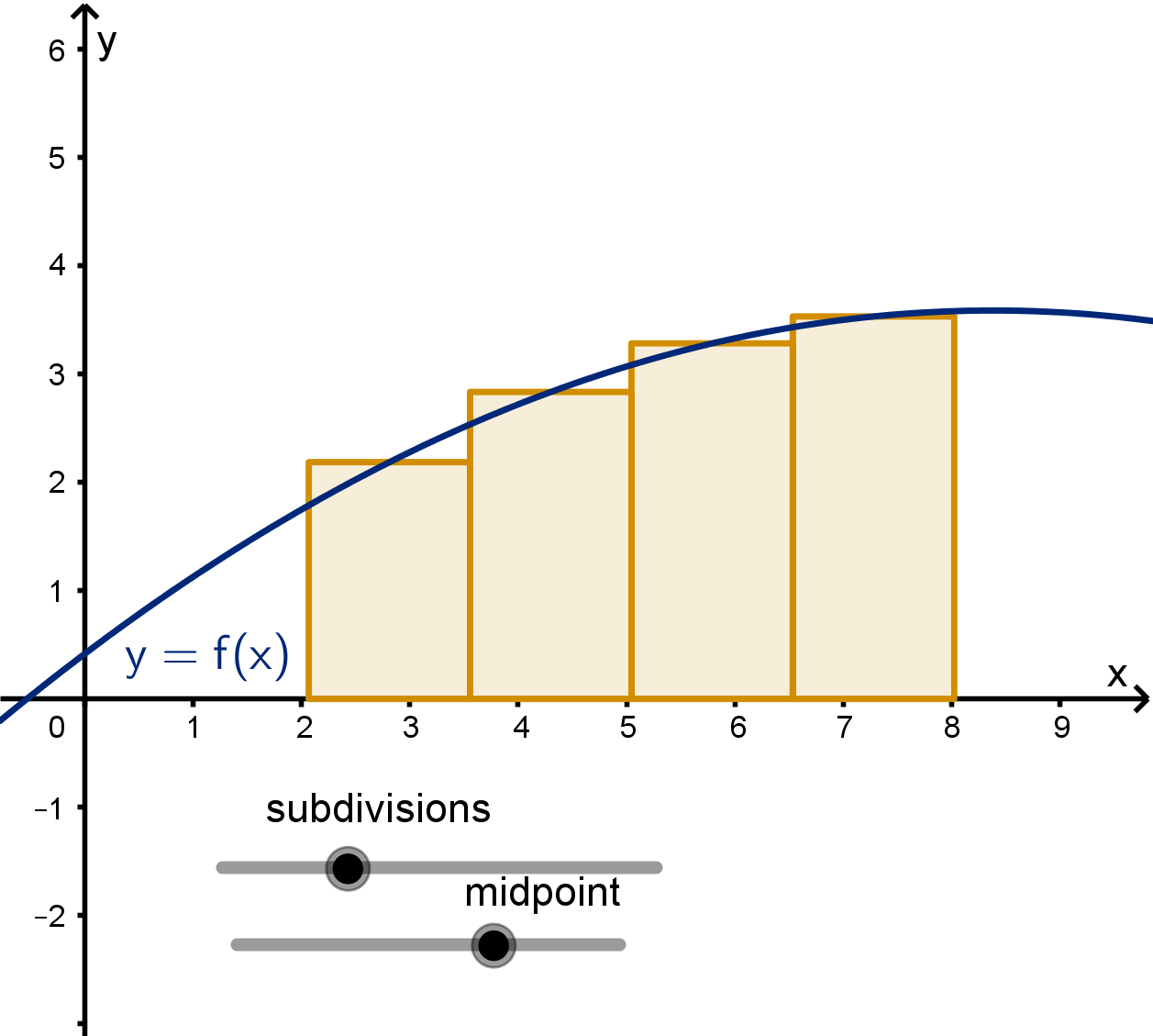
Figure: Approximations of an integral and of a function
Many measurable quantities can be found to depend on the value of multiple inputs. These are
multivariable functions like z = F (x, y), where z is a function of two independent variables. Examples
appear in all the sciences
1 Chemistry: V =
nrt
P
2 Physics: F =
GMm
r
2
3 Economics: P = P
0
e
rt
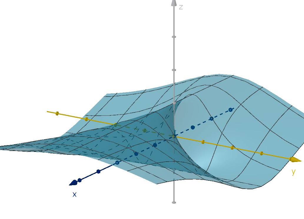
Figure: The graph of a two-variable function
We want to understand how to measure rates of change of these functions, and what these mea-
surements can do for us.
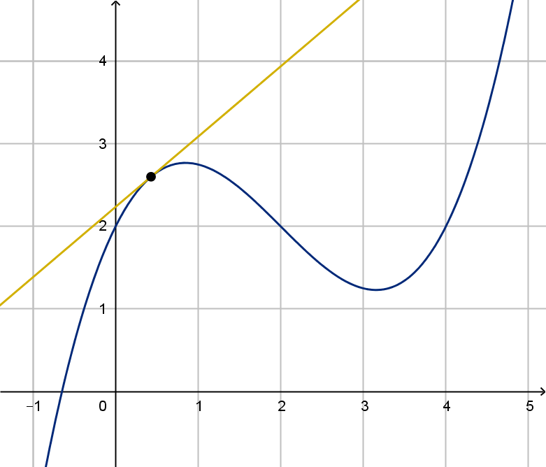
Furthermore, real world data does not come prepackaged with a differentiable function to describe
it. One approach is to find a line of best fit. Doing so requires optimizing two variables at once (slope
and intercept) to find the best fit.
3
Introduction
Figure: Fitting a line to a set of data points
The values of y may not be a function of x at all. Another view point is to see (x, y) as a randomly
chosen point in the plane. To model such random choices, we use a two-variable density function.
Volumes under its graph (computed by integrals) tell us where these random points are likely to lie.
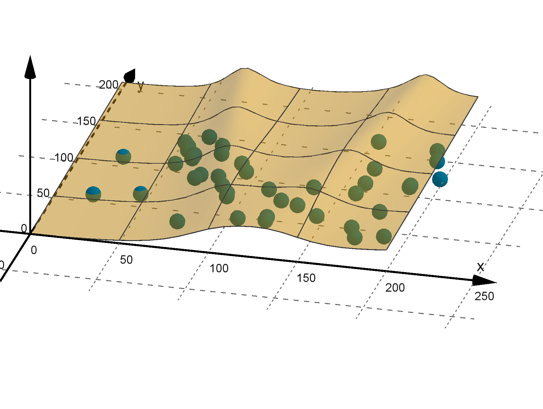
Figure: A function that models the outcomes of a random process
These approaches will requires us to use derivatives and integrals of multivariable functions.
4
Chapter 1
Review of Algebra and Calculus
This chapter reviews the most important information about functions, limits, derivatives, and integrals.
It is not meant to teach this material to a first-time learner, but can serve as a reference or reminder.
Contents
1.1 Graphs of Functions . . . . . . . . . . . . . . . . . . . . . . . . . . . . . . . 6
1.2 Limits and Derivatives . . . . . . . . . . . . . . . . . . . . . . . . . . . . . . 16
1.3 Applications of Derivatives . . . . . . . . . . . . . . . . . . . . . . . . . . . 35
1.4 Definite Integrals . . . . . . . . . . . . . . . . . . . . . . . . . . . . . . . . 44
Section 1.1
Graphs of Functions
Goals:
1 Graph algebraic and trigonometric functions.
2 Solve equations using inverse functions.
3 Solve equations containing quotients.
4 Graph transformations of functions.
Definition
The graph of an equation is the set of ordered pairs (x, y) that satisfy the equation. These are the
points that, when their coordinates are plugged in for x and y, the two sides of the equation are equal.
Linear Functions
Linear functions can be written in slope-intercept form:
f(x) = mx + b.
The graph y = mx + b of a linear function is a line.
m is the slope, which is the change in y over the change in x between any two points on the line.
(0, b) is the y intercept.
If we have the slope and a known point (x
0
, y
0
) on a line. We can write its equation in point-slope
form.
y −y
0
= m(x − x
0
)
If we have both the x- and y-intercepts of the line, it is convenient to write it in normal form
ax + by + c = 0
6
Monomials
A monomial is a function of the form:
f(x) = x
n
where n is an integer greater than 0.
For n ≥ 2 the graph y = x
n
curves upward over the positive values of x.
Higher values of n have lower values when 0 < x < 1 but higher values after x > 1.
For even values of n the graph is symmetric across the y-axis, curving up when x is negative.
For odd values of n the graph curves down when x is negative. It is anti-symmetric across the
x = 0.
Figure: Graphs of monomials of odd and even powers
Monomials of Negative Power
Monomials of negative power have the form f(x) = x
−n
. They are also commonly written
f(x) =
1
x
n
.
The graph y =
1
x
n
has a vertical asymptote at x = 0.
The graph approaches the x-axis, y = 0 as x gets large.
For even values of n, the graph is above the x-axis.
For odd values of n, the graph is above the x-axis for positive x and below it for negative x.
A larger choice of n makes the function approach the x-axis more quickly.
7
Section 1.1 Graphs of Functions
Figure: Graphs of monomials of negative odd and even powers
Roots
A root functiom is a function of the form:
f(x) =
n
√
x
where n is an integer greater than 0.
The domain of
n
√
x is [0, ∞) if n is even and all real numbers if n is odd.
The x and y intercept of y =
n
√
x is at (0, 0).
Root functions are increasing. At x = 0, they travel straight up.
Figure: The graphs of y =
√
x and y =
3
√
x
8
Exponential Functions
An exponential function has the form:
f(x) = a
x
where a is a number greater than 0.
a is called the base of the exponential function.
The graph y = a
x
passes through (0, 1).
If a > 1 then f(x) increases quickly as x takes on positive values. Higher values of a give a
steeper increase. f(x) approaches 0 as x goes to −∞. Higher values of a give a faster approach.
The graph does not touch or cross the x-axis.
If a < 1, then the above is reversed.
e is a commonly used base. e is approximately 2.718.
Figure: The graphs of exponential functions
Logarithms
A logarithmic function have the form:
f(x) = log
x
a
where a is a number greater than 1. log
a
x is the number b such that a
b
= x.
a
b
can never be 0 or less. The domain of f(x) = log
x
a
is (0, ∞).
As x goes to 0, log
a
x goes to −∞.
y = log
a
x has an x intercept at (1, 0).
9
Section 1.1 Graphs of Functions
Figure: The graphs of logarithm functions
Logarithms and exponents are inverse functions. We solve exponential equations by applying a
logarithm to both sides. We solve logarithm equations by exponentiating both sides.
a
x
= c x = log
a
c
log
a
x
= c x = a
c
Trigonometric Functions
f(x) = sin x and f (x) = cos x are periodic functions.
sin x and cos x have a range of [−1, 1].
These functions are periodic. This means that for all x, f(x + 2π) = f(x).
Figure: The graphs of y = sin x and y = cos x
10
The other trigonometric functions can be written in terms of sine and cosine.
tan x =
sin x
cos x
cot x =
cos x
sin x
sec x =
1
cos x
csc x =
1
sin x
Since trigonometric functions obtain the same values infinitely many times, the do not technically
have inverse functions. However, we define inverse trigonometric functions on a restricted range.
−
π
2
≤ sin
−1
x ≤
π
2
0 ≤ cos
−1
x ≤ π
−
π
2
≤ tan
−1
x ≤
π
2
These functions provide one solution to a trigonometric equation. We can obtain the others by using
the periodic behavior of trognometric funtions.
sin x = c x = sin
−1
c + 2πn or π − sin
−1
c + 2πn
cos x = c x = cos
−1
c + 2πn or − cos
−1
c + 2πn
tan x = c x = tan
−1
c + πn
Where n can be any integer.
Question 1.1.1
How Do Transformations Affect the Graph of a Function?
Transformations
Suppose we would like to transform the graph y = f(x). Here are four ways we can.
The graph of y = af(x) is stretched by a factor of a in the y direction.
The graph of y = f(x) + b is shifted by b in the positive y direction.
The graph of y = f(cx) is compressed by a factor of c in the x direction.
The graph of y = f(x + d) is shifted by d in the negative x direction.
11
Question 1.1.1
How Do Transformations Affect the Graph of a Function?
Figure: The graphs of y = f(x) and it transformation
Example 1.1.2
A Equation with Quotients
An equation of the form
f(x)
g(x)
= 0 is satisfied whenever f(x) = 0 but g(x) = 0.
Example
Solve
2x
2
− 3x − 5
x
2
+ 3x + 2
= 0
12
Solution
2x
2
− 3x − 5 = 0 set numerator = 0
(2x − 5)(x + 1) = 0 factor
x =
5
2
or x = −1
Then we must check that neither of these causes the denominator to be 0.
5
2
2
+ 3
5
2
+ 2 =
63
4
(−1)
2
+ 3(−1) + 2 = 0
So x =
5
2
is the only solution.
If there are terms besides the quotient, move them all to the same side of the equation and use a
common denominator to combine them.
Example
Solve
2 +
x + 3
x + 1
=
4
x
Solution
2 +
x + 3
x + 1
−
4
x
= 0 move to one side
2x
2
+ 2x
x
2
+ x
+
x
2
+ 3x
x
2
+ x
−
4x + 4
x
2
+ x
= 0 common denominator
3x
2
+ x − 4
x
2
+ x
= 0 combine
set 3x
2
+ x − 4 = 0
(3x + 4)(x − 1) = 0 factor
x = −
4
3
or x = 1
Then we must check that neither of these causes the denominator to be 0.
−
4
3
2
+
−
4
3
=
4
9
1
2
+ 1 = 2
Both solutions are valid. x = −
4
3
or x = 1.
13
Section 1.1
Exercises
1.1
Q1
Simplify
5
2
5
4
3
Q2
Simplify e
5
(e
4
)
3
Q3
Compress 2 log
5
x + log
5
y −3 log
5
z into a single logarithm.
Q4
Compress 3 ln(x + y) − ln(x
2
+ 2xy + y
2
) into a single logarithm.
Q5
Solve 2e
x
− 7 = 22
Q6
Solve 4 cos(2x) = 1
Q7
Solve 2 sin
2
x − 1 = 0
Q8
Solve 2 ln(x − 5) = 16
Q9
Solve 4
3x−2
= 15
Q10
Solve log
7
(x
2
+ 5) − 3 = 11
1.1.1
Q11
Graph y = 3 sin(2x).
Q12
Graph y = −ln x + 5.
Q13
Graph y = e
x
− 4.
Q14
Graph y =
3
√
x + 3.
Q15
Graph y =
1
(x − 2)
2
.
14
Q16
Graph y = −2
√
x + 1 + 4.
1.1.2
Q17
Solve for x:
x
2
+ 5x − 6
x − 1
= 0
Q18
Solve for x:
e
x
− 2
x
2
+ 2x − 3
= 0
Q19
Solve for x:
3x
2
− 5
2e
x
− 7
= 0
Q20
Solve for t:
ln t − 4
3 − t
= 0
Q21
Solve for x:
ln x − 4
3 − x
= 0
Q22
Solve for x:
3
x + 2
=
7
x + 4
Q23
Solve for u:
5
(u + 1)
2
=
u
u + 1
15
Section 1.2
Limits and Derivatives
Goals:
1 Compute limits of functions.
2 Verify that a function is continuous.
3 Compute derivatives.
4 Use derivatives to understand graphs and vice versa.
Question 1.2.1
What Is a Limit?
The Limit of a Function
If we can make f (x) arbitrarily close to some number L by considering only x in a small interval
(a, a + δ) then we say the limit of f as x approaches a from the right is L. We write:
lim
x→a
+
f(x) = L
If f(x) cannot be made arbitrarily close to any number, then this limit does not exist.
Similarly, if we can make f (x) arbitrarily close to some number L by considering only x in a small
interval (a − δ, a) then we say the limit of f as x approaches a from the left is L. We write:
lim
x→a
−
f(x) = L
If f(x) cannot be made arbitrarily close to any number, then this limit does not exist.
If both lim
x→a
+
f(x) = L and lim
x→a
−
f(x) = L, we say the two-sided limit or just limit of f as x
approaches a is L. We write
lim
x→a
f(x) = L
If the either the limit from the left or the limit from the right does not exist, or if they do exist
but are not equal to each other, then the two sided limit does not exist.
16
Figure: An interval of x values that produce values in a small neighborhood of L when plugged into
f(x).
Infinite Limits
If f(x) can be made arbitrarily large by considering only x in a small interval (a, a + δ) then we say the
limit of f as x approaches a from the right is ∞.
lim
x→a
+
f(x) = ∞
This is a way of representing growth without bound. Infinite limits from the left are defined anal-
ogously. Also analogous is our treatment of a function then decreases without bound. We say these
functions limit to −∞. If either one-sided limit at x = a is infinite, then the line x = a is a vertical
asymptote of y = f(x).
Example
Let f(x) =
1
x
.
lim
x→0
+
f(x) = ∞
lim
x→0
−
f(x) = −∞
17
Question 1.2.1
What Is a Limit?
Figure: The graph of y =
1
x
Vertical Asymptotes
There are only two common algebraic constructions that produce infinite limits.
A function of the form
f(x)
g(x)
where lim
x→a
g(x) = 0 and lim
x→a
f(x) = 0.
lim
x→0
+
log
a
x = −∞.
Remark
∞ is not a number, so if lim
x→a
+
f(x) = ∞ we would still say that lim
x→a
+
f(x) does not exist.
There are several limit laws that allow us to compute limits of combinations of simpler functions.
Theorem [Limit Laws]
The following hold limits, provided that lim
x→a
f(x) and lim
x→a
g(x) exist.
lim
x→a
(f(x) + g(x)) = lim
x→a
f(x) + lim
x→a
g(x)
lim
x→a
(cf(x)) = c lim
x→a
f(x)
lim
x→a
(f(x)g(x)) =
lim
x→a
f(x)
lim
x→a
g(x)
lim
x→a
f(x)
g(x)
=
lim
x→a
f(x)
lim
x→a
g(x)
!
provided that lim
x→a
g(x) = 0
lim
x→a
f(g(x)) = lim
x→b
f(x) provided that lim
x→a
g(x) = b
We can write similar statements for one-sided limits, though we need to be careful about directions in
the composition rule.
18
Question 1.2.2
What is Continuity?
Definition
A function f(x) is continuous at a, if
lim
x→a
f(x) = f(a)
Remark
This definition is useful, if we already know we are dealing with a continuous function. For example
f(x) = sin x is continuous so
lim
x→
π
6
sin x = sin
π
6
=
1
2
Fortunately, many familiar functions are continuous.
Theorem
The following functions are continuous on their domains
1 Constant functions
2 Linear functions
3 Polynomials
4 Roots
5 Exponential functions
6 Logarithms
7 Trigonometric functions
8 f(x) = |x|
More complex functions made from continuous functions are also continuous.
19
Question 1.2.2
What is Continuity?
Theorem
If f(x) and g(x) are continuous on their domains, and c is a constant, then the following are also
continuous on their domains
1 f(x) + g(x)
2 f(x) − g(x)
3 f(x)g(x)
4
f(x)
g(x)
(note that any x where g(x) = 0 is not in the domain)
5 f(x)
g(x)
as long as f(x) > 0
6 f(g(x))
Remark
Putting the above theorems together, we see that just about any function we can write using alge-
braic and trigonometric expressions is continuous on its domain. This does not mean it is continuous
everywhere. f(x) =
1
x
is not continuous at x = 0, for example.
Example 1.2.3
Computing a Limit
How do we compute lim
x→3
x
2
− 7x + 12
x − 3
?
Solution
f(x) =
x
2
−7x+12
x−3
is continuous on its domain, but x = 3 is not in the domain. However, let g(x) = x−4.
We know
x
2
−7x+12
x−3
= x − 4 for every x except x = 3. Specifically, in any neighborhood around x = 3,
f(x) = g(x) so they have the same limit.
lim
x→3
x
2
− 7x + 12
x − 3
= lim
x→3
x − 4 because they agree around x = 3
= 3 − 4 because g(x) = x − 4 is continuous at x = 3
= −1
20
Question 1.2.4
What Is the Intermediate Value Theorem?
One early intuition for continuity is that the graph of the function can be drawn without any breaks.
There are many ways to formalize this idea. One of the most important is the following theorem.
Theorem [The Intermediate Value Theorem]
If f is a continuous function on [a, b] and K is a number between f (a) and f(b), then there is some
number c between a and b such that f (c) = K.
This theorem essentially states that a continuous graph cannot get from one side of the line y = K
to the other without intersecting y = K. Notice that this theorem does not say exactly where this
intersection must occur, only that it must occur somewhere in the interval (a, b). It also does not rule
out the possibility of more than one such c existing.
Example
Show that f(x) = e
x
− 3x has a root between 0 and 1.
Solution
A root is a number c such that f(c) = 0. To prove such a root exists, we check the conditions of the
IVT.
f(x) is a sum of continuous functions, so it is continuous on its domain.
f(0) = 1
f(1) = e − 3 < 0
0 is between f(0) and f(1)
We conclude there is some c between 0 and 1 such that f(c) = 0.
21
Question 1.2.5
What Is a Limit at Infinity?
Definition
If we can make f(x) arbitrarily close to some number L by considering only x in some interval
(n, ∞) then we say the limit of f as x approaches ∞ is L. We write:
lim
x→∞
f(x) = L
If f(x) cannot be made arbitrarily close to any number, then this limit does not exist.
Similarly if we can f(x) arbitrarily close to L by considering only x in some interval (−∞, n) then
we say the limit of f as x approaches −∞ is L. We write:
lim
x→−∞
f(x) = L
If either lim
x→∞
f(x) = L or lim
x→−∞
f(x) = L, then y = L is a horizontal aysmptote of the graph
y = f(x).
By observing graphs or using arithmetic intuition, we arrive at the following limits at infinity.
f(x) lim
x→∞
f(x) lim
x→−∞
f(x) Comments
x
n
(n odd) ∞ −∞ n > 0
x
n
(n even) ∞ ∞ n > 0
n
√
x (n odd) ∞ DNE domain is x ≥ 0
n
√
x (n even) ∞ −∞
1
x
n
0 0 n > 0
a
x
(a > 1) ∞ 0
a
x
(0 < a < 1) 0 ∞
log
a
x ∞ DNE a > 1, domain is x > 0
sin x DNE DNE oscillates
tan
−1
x
π
2
−
π
2
22
Question 1.2.6
How Do We Measure the Change in a Function?
Definition
The average rate of change of a function f(x) between x = a and x = b is
f(b) − f(a)
b − a
This is also the slope of the secant line from (a, f(a)) to (b, f (b)) on the graph y = f(x).
Knowing the average rate of change over a range of inputs (or times) doesn’t tell us the rate of
change at a specific point (or moment). Geometrically the is the slope of the tangent line to y = f(x)
at a particular point (a, f(a))
Figure: A secant line and a tangent line
The secant lines get closer and closer to the tangent line (in slope) as b gets closer to a. This
suggests that we could take the limit of these approaching values to get the actual slope.
Definition
The instantaneous rate of change or derivative of a function f(x) at x = a is
lim
h→0
f(a + h) − f(a)
h
provided that this limit exists. This is also the slope of the tangent line to y = f (x) at (a, f (a)). Two
common notations for the derivative are
Prime notation: f
′
(a)
Leibniz notation:
df
dx
x=a
23
Question 1.2.6
How Do We Measure the Change in a Function?
Figure: A limit of the slopes of secant lines
We can attempt to compute the derivative at any point a. We can put these values together to
create a function f
′
(x).
Definition
The derivative function of f(x) is the function that takes the value
f
′
(x) = lim
h→0
f(x + h) − f(x)
h
at each x.
We can denote the derivative function as f
′
(x) or
df
dx
. The second can be rewritten
d
dx
f to emphasize
that we are applying the differentiation operation to the function f.
Example
If f(x) = x
2
+ 2x, compute f
′
(x).
24
Solution
f
′
(x) = lim
h→0
f(x + h) − f(x)
h
definition of derivative
= lim
h→0
(x + h)
2
+ 2(x + h) − x
2
− 2x
h
plug in x and x + h
= lim
h→0
x
2
+ 2xh + h
2
+ 2x + 2h − x
2
− 2x
h
distribute
= lim
h→0
2xh + h
2
+ 2h
h
cancel
= lim
h→0
2x + h + 2 functions agree except at h = 0 so limits are equal
= 2x + 0 + 2 limit = value on a continuous function
= 2x + 2
Theorem
If f
′
(x) > 0 for all x in some interval [a, b] then f(x) is increasing on [a, b].
If f
′
(x) < 0 for all x on [a, b] then f(x) is decreasing on [a, b].
We can take higher order derivatives by taking derivatives of derivatives. The derivative function
of f in this context is called the first derivative. Its derivative function is the second derivative. The
second derivative’s derivative function is the third derivative and so on.
Notation
The following notations are used for higher order derivatives
name prime notation Leibniz notation
first derivative f
′
(x)
df
dx
second derivative f
′′
(x)
d
2
f
dx
2
third derivative f
′′′
(x)
d
3
f
dx
3
fourth derivative f
(4)
(x)
d
4
f
dx
4
fifth derivative f
(5)
(x)
d
5
f
dx
5
25
Question 1.2.6
How Do We Measure the Change in a Function?
The sign of a higher order derivative tells us how the derivative of one order lower is changing. For
example if
d
5
f
dx
5
< 0, then
d
4
f
dx
4
is decreasing. The sign of higher order derivatives is difficult to discern
from the shape of y = f(x), with the exeption of the second derivative.
Theorem
If f
′′
(x) > 0 on some interval, then y = f (x) is concave up on that interval. If f
′′
(x) < 0, then
y = f(x) is concave down.
Definition
A point a such that f(x) is concave up to one side of a and concave down to the other side is called
an inflection point.
Question 1.2.7
How Do We Compute Derivatives
The limit definition of a derivative is too unwieldy to use every time. A better approach is to learn
the derivatives of some simple functions, and then use theorems to compute derivatives when those
functions are combined.
Derivatives of Simple Functions
d
dx
c = 0 (derivative of a constant is 0)
d
dx
x
n
= nx
n−1
for any n = 0 (The Power Rule)
d
dx
sin x = cos x
d
dx
cos x = −sin x
d
dx
e
x
= e
x
d
dx
a
x
= a
x
ln a for a > 0
d
dx
ln x =
1
x
26
Theorem
The following rules allow us to differentiate functions made of simpler functions whose derivative we
know.
Sum Rule (f(x) + g(x))
′
= f
′
(x) + g
′
(x)
Constant Multiple Rule (cf(x))
′
= cf
′
(x)
Product Rule (f(x)g(x))
′
= f
′
(x)g(x) + g
′
(x)f(x)
Quotient Rule
f(x)
g(x)
′
=
f
′
(x)g(x)−g
′
(x)f(x)
(g(x))
2
unless g(x) = 0
Chain Rule (f(g(x))
′
= f
′
(g(x))g
′
(x)
Example
Compute
d
dx
tan(x)
Solution
tan x =
sin x
cos x
. We apply the quotient rule
(tan x)
′
=
(sin x)
′
cos x − (cos x)
′
sin x
cos
2
x
quotient rule
=
cos
2
x + sin
2
x
cos
2
x
=
1
cos
2
x
Pythagorean identity
= sec
2
x
27
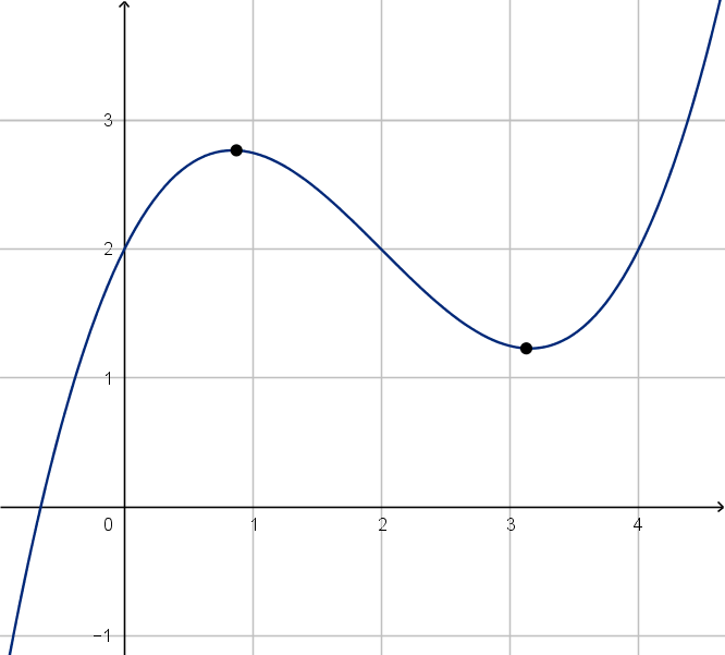
Application 1.2.8
The Shape of a Graph
What can the first and second derivative of f(x) = 8x
3
− x
4
tell us about the shape of its graph?
Solution
We will compute the first and second derivative using the power rule. Factoring them will allow us to
perform a sign analysis.
f
′
(x) = 24x
2
− 4x
3
f
′′
(x) = 48x − 12x
2
= 4x
2
(6 − x) = 12x(4 − x)
4x
2
+ + +
(6 − x) + + −
f
′
(x) + + −
0 6
12x − + +
(4 − x) + + −
f
′′
(x) − + −
0 4
From the sign of f
′
(x) we conclude f is increasing on (−∞, 0) and (0, 6) but decreasing on (6, ∞).
From the sign of f
′′
(x) we conclude that f is concave down on (−∞, 0) and (4, ∞), but concave up
on (0, 4).
Figure: The graph of y = 8x
3
− x
4
28
Section 1.2
Exercises
1.2.1
Q1
Given the graph of y = f(x) here, give the value of each of the following limits (if they exist).
a
lim
x→−3
−
f(x)
b
lim
x→−3
+
f(x)
c
lim
x→−2
f(x)
d
lim
x→0
f(x)
e
lim
x→4
−
f(x)
f
lim
x→4
+
f(x)
Q2
Given the graph of y = g(x) here, give the value of each of the following limits (if they exist).
a
lim
x→0
−
g(x)
b
lim
x→0
+
g(x)
c
lim
x→0
g(x)
d
lim
x→3
−
g(x)
e
lim
x→3
+
g(x)
f
lim
x→3
g(x)
g
lim
x→−4
−
g(x)
h
lim
x→−4
+
g(x)
i
lim
x→−1
g(x)
29
Section 1.2
Exercises
1.2.2
Q3
Explain why f(x) =
e
x
x
2
+3
is continuous on R.
Q4
Explain why f(x) =
p
sin(3x
2
) is continuous on its domain.
Q5
Is
f(x) =
sin(2x) if x < 0
4 if x = 0
−x
2
if x > 0
continuous at x = 0? Justify your answer.
Q6
Is
f(x) =
(
x
3
− 2x + 1 if x < 0
e
x
if x ≥ 0
continuous at x = 0? Justify your answer.
Q7
Is
f(x) =
x + 5 if x < 1
6 if x = 1
x
2
+ 4x + 1 if x > 1
continuous at x = 1? Justify your answer.
Q8
Where is
f(x) =
cos(πx) if x < 4
1 if x = 4
√
x − 3 if x > 4
continuous?
30
1.2.3
Q9
Compute lim
x→3
x − 3
x
2
− 9
Q10
Compute lim
x→1
x
2
− 4x + 3
x − 1
Q11
Compute lim
x→9
2x − 18
√
x − 3
Q12
Compute lim
x→4
1
x
2
−
1
16
x − 4
1.2.4
Q13
Explain why sin x = 2x − 1 has a solution in [0, 1].
Q14
Explain why
3
√
x = log
2
x has a solution in [0, 8].
Q15
What does the Intermediate Value Theorem say about whether f(x) =
1
x
−
1
2
has a root in
[−1, 1]?
Q16
Consider the equation sin x =
3
4
. Gloria computes sin
π
3
=
√
3
2
and sin
5π
6
=
1
2
. Since
3
4
is not
between
1
2
and
√
3
2
, she concludes that sin x =
3
4
has no roots in
π
3
,
5π
6
. What do you think
of Gloria’s reasoning?
1.2.5
Q17
Compute lim
x→∞
x
2
+ 2x − 9
3x − 6
.
Q18
Compute lim
x→∞
4x
2
− 7x + 9
2x
2
+ 11
.
Q19
Compute lim
x→∞
p
e
1/x
.
Q20
Compute lim
x→∞
1
ln x
.
31
Section 1.2
Exercises
Q21
Compute lim
x→−∞
e
e
x
.
Q22
Compute lim
x→∞
sin(ln x).
1.2.6
Q23
Let f(x) = x
3
.
a
Compute the average rate of change of f from x = 2 to x = 5.
b
Give the equation of the secant line that meets y = f(x) at x = 2 and x = 5.
c
Use the limit definition of the derivative to compute f
′
(2).
Q24
Let f (x) =
√
x Compute the average rate of change of f between x = 4 and x = 9. Based on
the graph of y = f(x), is the instantaneous rate of change at x = 4 greater or less than this
average?
Q25
Let f(x) = 3x
2
− 7. Compute f
′
(6) using the limit definition of the derivative.
Q26
Let f(x) =
1
x+2
. Compute f
′
(1) using the limit definition of the derivative.
Q27
Let f(x) =
1
x
2
. Compute f
′
(x) using the limit definition of the derivative.
Q28
Let f(x) =
√
x. Compute f
′
(x) using the limit definition of the derivative.
32
1.2.7
Q29
Use derivative rules to differentiate each of the following functions.
a
5x
7
− 3x
2
+
5
x
2
b
4x
5
− 2x
2
+ 3x + 4
x
c
(x
2
+ 2x) sin x
d
e
x
x
2
e
√
x − 5
f
cos(4x)
g
sin(e
x
)
h
(x
2
+ 5x + 4)
60
i
e
x
2
sin x
j
ln(x
2
+ 2)
x
2
+ 3x
Q30
Use derivative rules to differentiate each of the following functions.
a
3
x
+
7
x
3
b
5x
4
+ 3x
3
− 8x
2
x
2
c
ln x
x
d
4
x
sin(x)
e
tan(2x + 7)
f
e
3x+2
g
cos(x
3
+ 2x)
h
5
(cos x)
3
i
e
x
2
sin
3
x
j
ln(
√
x sin x)
Q31
Let f(x) = sin(3x). Compute f
′′′
(x).
Q32
Let f(x) = e
x
3
. Compute f
′′
(x).
1.2.8
Q33
Where in its domain is the function f(x) = x
3
− x
2
increasing?
33
Section 1.2
Exercises
Q34
Where in its domain is f(x) = e
x
− x
2
concave up?
Q35
Where in its domain is f(x) = 1024
√
x − x
4
increasing?
Q36
Find the inflection point(s) of x
4
− 8x
3
.
34
Section 1.3
Applications of Derivatives
Goals:
1 Write the equation of a tangent line.
2 Identify local maximums and minimums.
3 Use the Extreme Value Theorem to find minimums and maximums.
4 Use l’Hˆopital’s rule to compute limits.
This section reviews the most important applications of the derivative.
Application 1.3.1
The Tangent Line to a Graph
Given a function f (x), the derivative f
′
(a) is the slope of the line tangent to y = f(x) at (a, f(a)).
Formula
The equation of the tangent line to y = f(x) at x = a in point-slope form is:
y −f(a) = f
′
(a)(x − a)
We can rewrite the tangent line as a function of x. We call this a linearization, because this function
is linear, but it approximates the value of f(x) for x near a.
Formula
The linearization of y = f(x) at x = a is the function:
L(x) = f(a) + f
′
(a)(x − a)
If we want to emphasize the change in x and y instead of their actual values we can use differential
notation:
35
Application 1.3.1
The Tangent Line to a Graph
Notation
If y = f(x) is approximated by a tangent line at x = a then we let
dx = x − a represents a change in x from a. Since x is an independent variable, so is dx.
dy = f
′
(a) dx is equal to the change in y corresponding to dx, if we travel along the tangent
line. This approximates the actual change in f(x) if x increases by dx.
Figure: The differentials dx and dy on the tangent line to y = f (x)
Application 1.3.2
Maximum and Minimum Values of a Function
Definition
A number a is a maximum of a function f(x) if f(a) ≥ f(x) for all x in the domain of f.
a is a minimum if f(a) ≤ f(x) for all x in the domain of f.
36
Definition
A number a is a local maximum of a function f(x) if f (a) ≥ f(b) for all b in some neighborhood of a.
a is a local minimum if f(a) ≤ f(b) for all b in some neighborhood of a.
To distinguish ordinary maximums from the local variety, we sometimes call them global maximums
or absolute maximums. Every global maximum is a local maximum, but local maximums need not be
global maximums. If f
′
(a) > 0 then there are larger values of f(a) to the right of a and lower values
to the left. Thus a cannot be a local maximum or minimum. The same argument applies if f
′
(a) < 0.
Figure: Maximum and minimum values of f(x)
Definition
A critical point of f(x) is a value a in the domain of f such that either f
′
(a) = 0 or f
′
(a) does not
exist.
Theorem [The First Derivative Test]
Local maximums and minimums of f(x) can only occur at critical points.
We can use concavity as a way to classify critical points. Knowing whether a graph is concave up
or concave down at a point where f
′
(x) = 0 allows us to visualize a small neighborhood of that point.
37
Application 1.3.2
Maximum and Minimum Values of a Function
Theorem [The Second Derivative Test]
Let a be a critical point of f.
If f
′′
(a) < 0 then a is a local maximum.
If f
′′
(a) > 0 then a is a local minimum.
If f
′′
(a) = 0 or does not exist, then the test is inconclusive. a could be a local maximum, a local
minimum, or neither.
Example
What does the second derivative test tell you about the critical points of f(x) = 8x
3
− x
4
?
Solution
First we compute the critical points.
f
′
(x) = 24x
2
− 4x
3
compute first derivative
0 = 24x
2
− 4x
3
set equal to 0
0 = 4x
2
(6 − x) factor
x = 0 or x = 6
Now we compute the second derivative and evaluate it at each critical point.
f
′′
(x) = 48x − 12x
2
f
′′
(0) = 0
f
′′
(6) = (48)(6) − (12)(36) = −144
f
′′
(6) < 0 so x = 6 is a local maximum. f
′′
(0) = 0 so the second derivative test cannot tell whether
x = 0 is a local maximum or local minimum (in fact it is neither).
38
Question 1.3.3
Does a Function Always Have a Maximum?
No. Many functions don’t have maximums, because as x gets larger and larger the values of f(x)
increase or decrease without bound. However, if we restrict the domain, we can sometimes guarantee a
maximum
Theorem [The Extreme Value Theorem]
If f(x) is a continuous function on a closed domain [a, b] then f has an absolute maximum and an
absolute minimum on [a, b].
Remark
When the EVT applies, we can find the absolute maximum and minimum by process of elimination. A
maximum exists, so it must occur at a critical point. We can find the critical points and evaluate f at
each of them. Whichever has the greatest value is the maximum.
Note that a and b are always critical points because the derivative does not exist there. There is no
limit from the left at a because those points are outside the domain of f. Similarly, there is no limit
from the right at b.
Example
Compute the maximum and minimum value of f(x) = 8x
3
− x
4
on the domain [2, 8], if they exist.
Solution
f(x) is continuous and [2, 8] is closed, so the EVT guarantees that a maximum and minimum exist.
The first derivative test says that they can only occur at critical points.
f
′
(x) = 24x
2
− 4x
3
compute first derivative
0 = 24x
2
− 4x
3
set equal to 0
0 = 4x
2
(6 − x) factor
x = 0 or x = 6
x = 0 is not in the domain, so we discard it. On the other hand x = 2 and x = 8 are also critical points
because the derivative does not exist there. To find which critical point is the maximum and which is
the minimum, we plug each into f and compare.
f(2) = (8)(8) − 16 = 48
f(6) = (8)(216) − 1296 = 436 (maximum)
f(8) = (8)(512) − 4096 = 0 (minimum)
39
Application 1.3.4
L’Hˆopital’s Rule
The limit rules tell us how to take limits of quotients, products, sums and differences. What happens
if one of the functions being divided goes to ∞, or if the denominator of a quotient goes to 0? In some
cases we can reason this out using our intuition of arithmetic.
Example
Consider lim
x→∞
tan
−1
(x)
ln x
.
lim
x→∞
tan
−1
x =
π
2
lim
x→∞
ln x = ∞
Since the numerators are approaching π/2 and the denominators are increasing without bound, we
conclude that this ratio get smaller and smaller and will limit to 0.
In other cases, intuition cannot help us.
Definition
A limit of the form lim
x→a
f(x)
g(x)
is of indeterminate form if either
lim
x→a
f(x) = ±∞ and lim
x→a
g(x) = ±∞ or
lim
x→a
f(x) = 0 and lim
x→a
g(x) = 0
This definition also applies to one-sided limits or to limits at ±∞.
Limits of products and sums can sometimes be rewritten as quotients of indeterminate form as well.
Theorem [L’Hˆopital’s Rule]
If lim
x→a
f(x)
g(x)
is of indeterminate form, then it is equal to
lim
x→a
f
′
(x)
g
′
(x)
assuming this limit exists.
Often L’Hˆopital’s Rule converts a limit of indeterminate form to one we can evaluate through intuition
or direct computation. Sometimes, we need to apply L’Hˆopital’s Rule more than once.
Warning
If a limit is not of indeterminate form, then L’Hˆopital’s Rule does not apply. Attempting to apply it will
usually give an incorrect value for the limit.
40
Example 1.3.5
A Limit of Indeterminate Form
Evaluate lim
x→0
e
x
− x − 1
x
2
Solution
lim
x→0
e
x
− x − 1
x
2
0
0
form
= lim
x→0
e
x
− 1
2x
L’Hˆopital’s Rule, still
0
0
form
= lim
x→0
e
x
2
L’Hˆopital’s Rule again
=
1
2
Section 1.3
Exercises
1.3.1
Q1
Write the equation of the tangent line to y =
√
x at (4, 2).
Q2
Write the equation of the tangent line to y =
1
x
2
at
5,
1
25
.
Q3
Let f(x) = sin(x)
a
Write the equation of the linearization y = f(x) at x =
π
3
.
b
If we wanted to use
a
to approximate sin(1) by hand, what number(s) would we need
decimal approximations of?
c
Use a calculator to get decimal approximations of those numbers, then show how to approx-
imate sin(1).
Q4
Write a linearization of f(x) =
1
x
at x = 3 and use it to approximate
1
2.93
.
41
Section 1.3
Exercises
Q5
A baterical culture has mass 3g after t = 5 hours of growth. At that time, its instantaneous rate
of growth is 0.2g/hr.
a
Write a linear function to approximate m(t) the mass of the culture at hour t.
b
Approximate the mass at time 8 hours.
c
Given that m
′′
(t) > 0, is your answer to
b
is overestiamte or an underestimate?
Q6
A space capsule is descending from orbit. After 90 seconds, it is 10, 000m above sea level and
falling at 400m per second.
a
Write a linearization for h(t), the height of the capsule at time t.
b
Use
a
to predict when the capsule will splash down into the ocean.
c
Do you expect that your answer to
b
is an overestimate or underestimate? Explain.
1.3.2
Q7
Find the critical points of f(x) = 12x
2/3
− x.
Q8
Find the critical points of g(x) = x
4
− 18x
2
+ 5. Apply the second derivative test to each.
Q9
Find the critical points of f(x) = x
3
− 75x. Apply the second derivative test to each.
Q10
Find the critical points of g(x) = e
x
− 2x. Apply the second derivative test to each.
1.3.3
Q11
Find the maximum and minimum values of f(x) = x
2/3
on [−8, 1].
Q12
Find the maximum and minimum values of f(x) = x
3
− 75x on [−10, 10].
42
1.3.4
Q13
Evaluate lim
x→0
+
x cos(x − π)
e
x
− 1
.
Q14
Evaluate lim
x→0
+
e
−3x
+ 3x − 1
sin(x
2
)
.
Q15
Evaluate lim
x→∞
x ln x
x
5/2
+ 3
.
Q16
Evaluate lim
x→−∞
e
x
x
2
.
43
Section 1.4
Definite Integrals
Goals:
1 Express areas under a graph and antiderivatives using integral notation.
2 Derive antiderivatives from known derivatives.
3 Compute general antiderivatives.
4 Compute definite integrals using the Fundamental Theorem of Calculus.
5 Use u-substitution to compute integrals where necessary.
By definition, integrals compute area under a graph. The Fundamental Theorem of Calculus connects
integrals to antiderivatives, meaning that integrals can also be used to compute total change, given a
rate of change function.
Question 1.4.1
What Is an Antiderivative?
Definition
F (x) is antiderivative of a function f(x), if F
′
(x) = f(x).
Every derivative we know also tells us an antiderivative.
Example
d
dx
x
2
2
+ 5
= x so F (x) =
x
2
2
+ 5 is an antiderivative of f(x) = x.
Notice that
x
2
2
+ 2,
x
2
2
− 6, and
x
2
2
are also antiderivatives of f(x) = x.
Functions have infinitely many antiderivatives. Adding a constant to one antiderivative produces
another, since the derivative of a constant is 0. In fact, this is the only relationship between antideriva-
tives.
Theorem
If F (x) and G(x) are antideriavatives of f(x), then there is a constant c such that
F (x) = G(x) + c.
Since the antiderivatives are related this way, it is easy to express all of the antiderivatives of a
function at once.
44
Definition
If F (x) is an antiderivative of f(x), then the general antiderivative of f(x) is the family of functions:
F (x) + c
where c can be any constant.
Here is a table of antiderivatives that we can compute just by reverse engineering the derivatives we
already know.
f(x) general antiderivative of f(x)
x
n
x
n+1
n+1
+ c
e
x
e
x
+ c
a
x
a
x
ln a
+ c
1
x
ln x + c
sin x −cos x
cos x sin x
Remark
Many familiar functions are missing from this list. This is because we just haven’t come across them as
derivatives of some other function. For instance, we do not yet know a function F (x) whose derivative
is ln x or tan x.
Question 1.4.2
How Do We Compactly Denote a Sum of Many Terms
Defining the definite integral requires us to add up many numbers. The problem is not just that
the number of summands is large. We need to be flexible about how many terms are in the sum. The
notation that gives us this flexibility is Σ notation.
Notation
Σ (‘sigma’) notation allows us to sum many different values of an expression using an index variable.
The index variable will be replaced by each integer between an initial and final value, and the resulting
outputs are added together.
n
X
k=1
f(k) = f(1) + f(2) + f(3) + ··· + f(n)
We may choose any variable as the index variable. The index variable could also have a different initial
value, if that is more convenient.
45
Question 1.4.2
How Do We Compactly Denote a Sum of Many Terms
Example
7
X
j=3
j
2
j + 1
=
9
4
+
16
5
+
25
6
+
36
7
+
49
8
Part of the challenge of writing a sum in
P
notation is choosing an f that will produce all the terms
of your sum.
Example 1.4.3
Writing a Sum in Σ Notation
Write each of the following sums in Σ notation.
a
4 + 7 + 10 + 13 + 16 + 19 + 22
b
2 + 6 + 18 + 54 + 162 + 486
c
−3 + 4 − 5 + 6 − 7 + 8 − 9 + 10
d
1
4
+
√
2
9
+
√
3
16
+
2
25
+
√
5
36
Solution
a
The terms increase by 3 each time. Repeated addition is multiplication, in this case 3k plus some
starting value. Starting with index k = 0 is convenient, because 3(0) = 0 at the starting value.
4 + 7 + 10 + 13 + 16 + 19 + 22 =
6
X
k=0
4 + 3k
b
The terms are multiplied by 3 each time. Repeated multiplication is exponentiation, in this case
3
k
times some starting value. Starting with index k = 0 is convenient, because 3
0
= 1 at the
starting value.
2 + 6 + 18 + 54 + 162 + 486 =
5
X
k=0
(2)(3
k
)
46
c
The absolute values of this sum could just be the values of the index variable. To create an
alternating + and − pattern, we can multiply by (−1)
k
.
−3 + 4 − 5 + 6 − 7 + 8 − 9 + 10 =
10
X
k=3
(−1)
k
k
d
In a fraction, we can model the numerator and denominator separately.
1
4
+
√
2
9
+
√
3
16
+
2
25
+
√
5
36
=
5
X
k=1
√
k
(k + 1)
2
Question 1.4.4
How Do We Compute the Area Under a Graph?
Suppose we would like to know the area below the graph y = f (x) between x = a and x = b. We
approximate this area by rectangles. We can improve these approximations and take a limit of such
improvements to compute the actual area. Here is the procedure.
1 Divide [a, b] into n subintervals, of lengths ∆x
i
.
2 Pick a point x
∗
i
in each subinterval.
3 Evaluate f(x
∗
i
), which is the height of the graph above x
∗
i
.
4 Produce a rectangle of height f(x
∗
i
) and width ∆x
i
over each subinterval.
5 Sum the areas of these rectangles. This is an approximation of the actual area.
6 Take a limit of such approximations as |∆x|, the largest of the ∆x
i
goes to 0.
Figure: The area under y = f(x) approximated by rectangles
47
Question 1.4.4
How Do We Compute the Area Under a Graph?
Defintion
We define the definite integral of f(x) over [a, b] to be
Z
b
a
f(x) dx = lim
|∆x|→0
X
f(x
∗
i
)∆x
i
where the limit is taken over all divisions of [a, b], ∆x
i
is the length of the ith subinterval, x
∗
i
is a point
in the ith subinterval and |∆x| is the largest ∆x
i
.
Notice there is no requirement that the subintervals be the same length. Because of this, we don’t
take a limit as n approaches ∞. For instance, using a large number of rectangles from
a,
a+b
2
and only
a single rectangle over
a+b
2
, b
will not give us a good approximation, no matter how many rectangles
we use. Instead we take a limit as the largest ∆x
i
approaches 0.
In practice, we get the same limit whether the subintervals are equal length or not not. It is common
to use the same ∆x =
b−a
n
for each subinterval.
The definite integral almost solves our area problem, but wherever f(x) < 0, the product f (x
∗
i
)∆x
i
will be negative.
Theorem
If f(x) > 0 on [a, b] then
Z
b
a
f(x) dx computes the area under y = f(x) over [a, b]. In general
Z
b
a
f(x) dx computes the signed area between y = f(x) and the x-axis, where area above the axis
counts as positive, and area below the axis counts a negative.
Since integrals are limits, they inherit two laws from limits. The third can be taken from geometry,
setting the area of a region equal to the sum of the areas of two subregions.
Integral Laws
Z
b
a
f(x) + g(x) dx =
Z
b
a
f(x) dx +
Z
b
a
g(x) dx (Sum Rule)
Z
b
a
cf(x) dx = c
Z
b
a
f(x) dx (Constant Multiple Rule)
Z
b
a
f(x) dx =
Z
c
a
f(x) dx +
Z
b
c
f(x) dx (Union Rule)
48
Question 1.4.5
How Do We Evaluate an Integral?
The limit form of an integral is usually impossible to evaluate directly. Instead we use a powerful
pair of theorems.
Theorem [The First Fundamental Theorem of Calculus]
Given a function f(x), let g(x) =
Z
x
a
f(t) dt. At any x where f is continuous, g
′
(x) = f(x).
To prove this, we use the definition of a derivative.
g
′
(x) = lim
h→0
g(x + h) − g(x)
h
= lim
h→0
R
x+h
a
f(t) dt −
R
x
a
f(t) dt
h
= lim
h→0
R
x+h
x
f(t) dt
h
union rule
As the interval [x, x+ h] shrinks, the values of f over that interval can be made arbitrarily close to f(x),
since f is continuous. Thus
R
x+h
x
f(t) dt approaches the area of a rectangle of height f (x) and width
h. Thus
lim
h→0
R
x+h
x
f(t) dt
h
= f(x)
Figure: g(x + h) − g(x) represented as an area
The main use of the First Fundamental Theorem of Calculus is to prove the Second Fundamental
Theorem of Calculus.
Theorem [The Second Fundamental Theorem of Calculus]
Let f(x) be a continuous function on [a, b]. If F (x) an antiderivative of f(x), then
Z
b
a
f(x) dx = F (b) − F (a)
49
Question 1.4.5
How Do We Evaluate an Integral?
This follows immediately from the First Fundamental Theorem. If we continue to define g(x) =
R
x
a
f(t) dt, then
Z
b
a
f(x) dx =
Z
b
a
f(x) dx −
Z
a
a
f(x) dx
= g(b) − g(a)
We know that g(x) is an antiderivative of f (x). If we instead pick a different antiderivative F (x), then
F (x) = g(x) + c, and
F (b) − F (a) = g(b) + c − (g(a) + c)
= g(b) − g(a)
=
Z
b
a
f(x) dx
Because we will be computing F (b) − F (a) frequently, we will develop the following shorthand.
Notation
The quantity F (b) − F (a) can be denoted
F (x)
b
a
This relationship between integrals and antiderivatives motivates the following vocabulary.
Notation
The general antiderivative of f(x) is also called an indefinite integral and is denoted
Z
f(x) dx.
50
Example 1.4.6
A Definite Integral
Compute
Z
5
2
x
2
dx
Solution
Z
5
2
x
2
dx =
x
3
3
5
2
=
5
3
3
−
2
3
3
=
125 − 8
3
= 39
Question 1.4.7
How Do We Apply the Chain Rule in an Antiderivative?
The chain rule states that
(f(g(x)))
′
= f
′
(g(x))g
′
(x).
The key insight here is to rewrite think of g as a variable, in addition to being a function of x. Typically
we rename it with a letter closer to the end of the alphabet, like u. The following substituion theorem
uses the chain rule to say that we can integrate with respect to u instead of x.
Theorem
If u(x) is a function of x, then
Z
b
a
f(u(x))u
′
(x) dx =
Z
u(b)
u(a)
f(u) du
This allows us to replace a complicated integrand in x with a simpler one in u. To correctly rewrite
the integral, the bounds must be updated to the corresponding values of u.
We can also apply this to indefinite integrals. If F is an antiderivative of f, then
Z
f(u(x))u
′
(x) dx =
Z
f(u) du
= F (u) + c
= F (u(x)) + c
The most common u substitutions are linear, where u = ax.
51
Question 1.4.7
How Do We Apply the Chain Rule in an Antiderivative?
Example
Compute
Z
sin 3x dx
Solution
We will perform a u substitution, using u = 3x.
Z
sin(3x) dx =
Z
1
3
sin u du
= −
1
3
cos u + c
= −
1
3
cos(3x) + c
u = 3x
du = 3 dx
1
3
du = dx
u-substitution
Note that we should express our antiderivatives in terms of the original variable (often x), not in
terms of u.
Figure: The graphs y = sin x, y = sin 3x their related tangent lines
Example 1.4.8
A u-substitution
Compute the integral:
Z
3
0
xe
x
2
dx
52
Solution
We start by looking for a candidate for u(x). Since we want the integrand to be f(u(x))u
′
(x), we
note u(x) should be the inner function in some composition. x
2
is the natural target. We attempt the
substituion, and hope that the remaining factors in the integrand can be expressed in terms of u
′
(x).
We see that our u
′
(x) dx is 2x dx. Since we only have an x dx in our integrand, we divide by 2.
Z
3
0
xe
x
2
dx =
Z
9
0
1
2
e
u
du
=
1
2
e
u
9
0
=
1
2
(e
9
− 1)
u = x
2
x = 0 ⇒ u = 0
du = 2x dx x = 3 ⇒ u = 9
1
2
du = x dx
u-substitution
Section 1.4
Exercises
1.4.1
Q1
Write two different anti-derivatives of f (x) = x + 5.
Q2
Write two different anti-derivatives of f (x) = x
3
− 6x
2
+
2
x
.
Q3
Write a general antiderivative of f(x) = 4 cos x + 6x
2
.
Q4
Suppose x
4
−sin(x
3
) is an antiderivative of f(x). Write three other antiderivatives of f (x). You
should do this without computing what f is.
Q5
If F (x) and G(x) are both antiderviatives of f(x), find the value b such that 3F (x) −bG(x) is
also an antiderivative of f(x).
Q6
Suppose F and G are both antiderivatives of f(x). Suppose further that F is an antiderivative
of F and G is an antiderivative of G. Describe the possible values of F(x) − G(x).
53
Section 1.4
Exercises
1.4.2
Q7
Evaluate
5
X
k=2
3k − 2
Q8
Evaluate
4
X
j=−1
j
2
− j
Q9
Write a formula for the value of
b
X
k=a
c.
Q10
We do not need to write a constant multiple rule for Σ notation because we already have one.
Explain what rules of mathematics tell us that
b
X
k=a
cf(k) = c
b
X
k=a
f(k).
Q11
Explain what’s wrong with the following notation:
k
X
k=1
3k
2
+
1
k
Q12
Consider the sum
n
X
k=1
1
2
k
for a few different values of n. Can you conjecture a formula for this
sum (it will depend on n).
1.4.3
Q13
Write the following sums in Σ notation.
a
3 + 7 + 11 + 15 + 19
b
6 + 12 + 24 + 48 + 96 + 192
c
3
4
−
4
5
+
5
6
−
6
7
+
7
8
−
8
9
.
Q14
Write the following sums in Σ notation.
a
5 − 15 + 25 − 35 + 45 − 55 + 65 − 75 + 85 − 95
54
b
1
4
+
4
16
+
9
64
+
16
256
+
25
1024
c
√
2 +
√
6 +
√
12 +
√
20 +
√
30 +
√
42 +
√
56.
1.4.4
Q15
Does
R
1
1/2
ln x dx compute the area under y = ln x over
1
2
, 1
? Explain.
Q16
Suppose
R
b
a
f(x) dx < 0. What does this tell you about the graph y = f(x)? Be specific.
Q17
Draw a careful graph of y =
√
x. Use 5 subintervals of [1, 11] to estimate the area beneath the
graph over [1, 11]. Use the left endpoints of each subinterval as the test points x
∗
i
.
Q18
Draw a careful graph of y = 3x. Use 3 subintervals of [2, 8] to estimate the area beneath the
graph, with the test points x
∗
i
being the left endpoints of each subinterval.
Q19
Draw the graph of y = 7. Use geometry to evaluate
R
3
87 dx.
Q20
Draw the graph of y =
x
3
+ 1. Use geometry to evaluate
R
−3
9
x
3
+ 1 dx.
1.4.5
Q21
Let g(x) =
R
x
5
f(t) dt. What is g
′
(8)?
Q22
Let g(x) =
R
x
2
cos t dt. Is g(x) increasing or decreasing at x = 3? Explain.
Q23
Suppose f(x) is an increasing function. Is
R
31
22
f
′
(x) dx positive or negative?
Q24
Suppose F (x) and G(x) are both antiderivatives of f(x). Given the following incomplete table
of values, compute
R
4
1
f(x) dx.
x 1 2 3 4 5 6
F (x) − 7 − 13 − 9
G(x) 3 − 9 − 10 5
55
Section 1.4
Exercises
Q25
Explain the difference between
Z
f(x) dx and
Z
b
a
f(x) dx in a few sentences.
Q26
Compute
Z
π
0
cos(x) dx. Explain the geometric meaning of your answer in a sentence or two.
1.4.6
Q27
Compute
Z
8
1
x −
3
x
dx.
Q28
Compute
Z
4
1
1
t
3/2
dt.
Q29
Compute
Z
e
x
− 6x
2
dx.
Q30
Compute
Z
0
t
1
3
e
x
+ 5 dx.
Q31
Compute
Z
√
t dt.
Q32
Compute
Z
2
10
x
2
+ 2
5x
dx.
Q33
Compute
Z
3
5
sin y dy.
Q34
Compute
Z
2
0
x
4
− 3x + 2 dx.
Q35
Compute
Z
3π/4
π/6
2 cos v dv.
Q36
Compute
Z
π
0
2 sin t + cos t dt.
56
1.4.7
Q37
Write some general rules. Suppose F (x) + c is the antiderivative of f(x)
a
What is the antiderivative of f(x + a)?
b
What is the antiderivative of f(ax)?
Q38
Assuming that
Z
b
a
f(x) dx exists, argue that it is equal to
Z
2b
2a
1
2
f
x
2
dx, in the following two
ways:
a
By appealing to an integration rule.
b
By describing the relationship between the graphs of y = f(x) and y = f
x
2
. A picture
might help.
1.4.8
Q39
Compute
Z
e
7x
dx.
Q40
Compute
Z
√
5x + 3 dx.
Q41
Compute
Z
cos
θ
3
dθ.
Q42
Compute
Z
(t − 2)
6
dt.
Q43
Compute
Z
1/4
0
sin(πt) dt.
Q44
Compute
Z
3
0
x
2
e
x
3
dx.
Q45
Compute
Z
(x
5
− 2x)(5x
4
− 2) dx.
Q46
Compute
Z
3π/4
π/4
cos(x)
1
sin
2
x
dx.
57
Section 1.4
Exercises
58