Hybrid Regularization for Random Feature Models

This blog post was written by Tony Maccagnano, Sarah Skaggs, Madeline Straus, and Advay Vyas and published with minor edits. The team was advised by Dr. Chelsea Drum. In addition to this website, the team has given a midterm presentation, filmed a poster blitz video, created a poster, published code, and worked on a manuscript.

Motivation and Background

Image classification is the process by which computer models learn to identify distinguishing features in images in order to recognize and categorize them effectively. As a result, it has many diverse applications in bioinformatics, 3D reconstruction, information extraction, and signal and image processing. In particular, the medical field has seen significant benefits from image classification, which has enabled earlier and more accurate diagnoses by detecting patterns that often elude the human eye and by helping to reduce the rate of misdiagnosis.

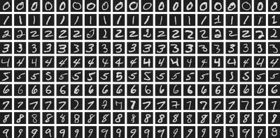
Two main problems within image classification are feature extraction and image labeling. For example, the image below represents photos of the widely studied MNIST dataset which contains handwritten digits 0-9. This dataset serves as a benchmark for training and evaluating classification models before applying them to real-world applications. A well-trained model should be able to efficiently and accurately classify each image as the correct digit before progressing to more complex and diverse classification problems.

Questions that we considered were:

• How exactly do computer models learn to identify the contents of an image?
• What happens when there is too much data for the computer system to handle?
• Can we improve the efficiency of existing classification methods?

Our Problem

A common and effective approach in image classification is to represent it as a large-scale linear inverse problem of the form $$B \approx AX$$ Here, $B$ is the observed output data (image labels), $A$ is the input image matrix and $X$ is the unknown coefficient matrix we want to approximate. This means we need to determine the input parameters of a system based on the output data. However, many systems are noisy and small disturbances in the label matrix can lead to large differences in the input data, meaning that our problem may be ill-posed. Additionally, when working with large datasets, solving this problem explicitly becomes computationally challenging. One effective strategy to address this is the use of random feature models.

Random Feature Models

Random feature models transform image data into a higher-dimensional space using randomly generated features, enabling the use of linear methods for classification or regression. A common challenge with this approach is the double descent phenomenon, where test error dips, then spikes, and then falls again as the number of features increases. The spike often appears when the number of features is close to the number of training images, because the system is at the interpolation threshold and becomes ill-conditioned.

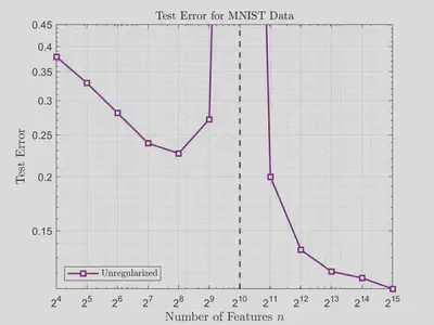
The figure below illustrates the double descent phenomenon when solving the problem directly without regularization. The test error spikes dramatically at $2^{10}$ features, which is also the number of images in this example.

Instead, we can regularize the problem to stabilize the solution and mitigate the effects of the double descent phenomenon.

We can either iteratively regularize the problem, meaning we solve it step by step on an increasing subspace, stopping when error is minimal, or we can do variational regularization, which involves solving a slightly different problem that incorporates the weights (complexity) of the solution. However, both of these approaches have their drawbacks. It can be difficult to know when to stop iterative regularization, while variational can take longer to converge and also requires us to provide a regularization parameter $\lambda$, and a bad one can negatively affect the accuracy of the model.

To get the benefits of these methods while mitigating their downsides, current research has combined the two into something called hybrid regularization. These methods use an iterative method to build the problem subspaces (e.g. Krylov) and apply variational regularization (e.g. Tikhonov) inside those subspaces.

Hybrid Regularization Methods

Previously, in [3], the hybrid LSQR method (available in MATLAB’s IR Tools package [2]) was successfully applied for the training of RFMs. Notably, the method:

• Avoided the double descent phenomenon
• Performed competitively against existing methods

However, this method uses computationally expensive inner products. Our proposal is to instead utilize a hybrid LSLU method, introduced in [1], which improves on hybrid LSQR by using a Hessenberg process that

• Does not require inner products
• Requires less storage and work

Through these improvements, this unique approach is advantageous for both mixed precision and high-performance computing scenarios.

Results and Conclusions

For our experiments, we tested various methods for the training of random feature models with the MNIST dataset. We specifically compared the hybrid LSLU method to hybrid LSQR and other standard regularized and unregularized methods.

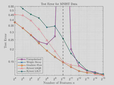
We compared test errors against the number of features for different methods on the MNIST dataset, which consists of $70,000$ images ($60,000$ training images, $10,000$ test images) of digits $0, 1, \dots, 9$, where each image is composed of $28 \times 28$ pixels. For this data we can take $n_i = 28 \times 28 = 784$ input features (a gray-scale level for each pixel), and $n_o = 10$ for the number of unique labels (digits). For the following results, we only utilize $2^{10}$ training images. The unregularized method clearly exhibits double descent, while the two simple regularization methods, weight decay and gradient flow have a clear, smooth convergence. However, weight decay and gradient flow require computation of the SVD. Hybrid LSLU and hybrid LSQR converge in a similar manner without requiring SVD.

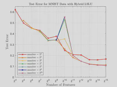
In the following figures, we plot test error against number of features for hybrid LSQR and hybrid LSLU on the MNIST data set for different numbers of iterations. We see here that while the accuracy with hybrid LSQR improves with increased iterations, the accuracy of hybrid LSLU is fairly stagnant across most values of features. We do observe that if too many iterations are utilized for hybrid LSLU, then the double descent phenomenon occurs.

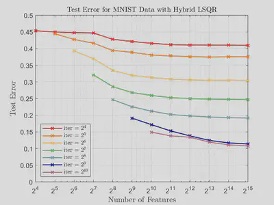
The following graphs show that hybrid LSLU converges much faster compared to hybrid LSQR in terms of number of iterations.

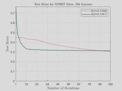
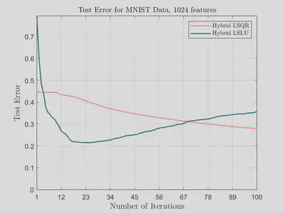
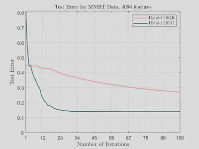
Our experiments show that hybrid LSLU converges much faster compared to hybrid LSQR in terms of number of iterations. Thus, not only is hybrid LSLU cheaper (in terms of computational cost) per iteration than hybrid LSQR, but it also requires less iterations to achieve comparable accuracy. We plan to investigate how to optimally stop hybrid LSLU in order to ensure the avoidance of the double descent phenomenon. In our future research we also hope to apply the randomized sketch-and-solve version of hybrid LSLU, which has the potential to address some of the issues we currently see.

Our Activities

Weeks 1 and 2

We did literature review on previous and current research. Using IRTools, we replicated the results of the pre-existing papers on hybrid LSQR by implementing random feature model projections.

Week 3

We composed our midterm presentation and began experimenting with the hybrid LSLU function and how it compared to hybrid LSQR.

Week 4

We worked on the midterm presentation and then researched different ways to optimize the regularization parameter λ.

Week 5

We looked more at double descent and different types of GCV in order to optimize LSLU with RFMs. We also started on the webpage draft.

Week 6

We put together our poster blitz video and started work on the manuscript while also working on getting results for the poster and manuscript. We researched more theory in order to properly explain our ideas.

Week 7

We put together our poster for the poster presentation and finalized our results and research. We implemented LSLU on MNIST and CIFAR10 and compared the test error to unregularized, weight decay, gradient flow and LSQR. We started working on the manuscript in order to get a rough draft done quickly.

Week 8

We presented our poster, finished up the manuscript, and cleaned up our code.

More about the Team

• Tony Maccagnano is a rising junior at Michigan Technological University, double majoring in Mathematics and Computer Science. He plans to go to graduate school for algebra or combinatorics.
• Sarah Skaggs is a rising junior at Virginia Tech double majoring in Computational Modeling and Data Analytics and Mathematics. She plans to go to graduate school for applied math and her dream career is to use math and data science to advance medical technology. Outside of academics, she loves to play pickleball, adventure, play board games and spend time with friends and family.
• Madeline Straus is a rising junior at Tufts University double majoring in Applied Mathematics and History, with plans to attend graduate school for math, and is particularly interested in numerical analysis and tomography. In her free time, she likes to read, compete at trivia, and play board games.
• Advay Vyas is a rising sophomore at the University of Texas at Austin double majoring in Statistics & Data Science and Mathematics. He hopes to pursue a PhD in Statistics and then work on new ideas in machine learning and its applications. In his free time, he loves to read novels, bike, and watch sports.

References and Further Reading

1. Ariana N Brown et al. “Inner Product Free Krylov Methods for Large-Scale Inverse Problems”. In: arXiv preprint arXiv:2409.05239 (2024).
2. Silvia Gazzola, Per Christian Hansen, and James G Nagy. “IR Tools: a MATLAB package of iterative regularization methods and large-scale test problems”. In: Numerical Algorithms 81 (2019), pp. 773–811.
3. Kelvin Kan, James Nagy, and Lars Ruthotto. “Hybrid Regularization Methods Achieve Near-Optimal Regularization in Random Feature Models”. In: Submitted to Transactions on Machine Learning Research (2024).
4. Ali Rahimi and Benjamin Recht. “Random Features for Large-Scale Kernel Machines”. In: Advances in Neural Information Processing Systems. Vol. 20. 2007, pp. 1177–1184