Learning Ordinary Differential Equations from Data
This post was written by Emma Hayes, Mathias Heider, and Carrie Vanty and published with minor edits. The team was advised by Dr. Deepanshu Verma.
In addition to this post, the team has also created slides for a midterm presentation, a poster blitz video, and a poster.
Project Overview:
Imagine a spring mass system (Figure 1). What if you wanted to find the location of the mass at any given time point? In order to find this information, you must first understand the dynamics of the system. A spring mass system is an example of simple harmonic motion where total energy is conserved. This means that you can model the dynamics using a Hamiltonian Ordinary Differential Equation, which has the quality of energy conservation. To solve our problem, we use neural networks utilizing Hamiltonians in the forward propagation to predict our coordinates.

Figure 1 - Spring Mass by Oleg Alexandrov (public domain)
Our project aims to compute the value of the Hamiltonian for any given time and set of initial conditions using Hamiltonian Inspired neural networks. We will first introduce the mathematical background of our project and the novel technique we implemented for our forward propagation. Results will then be presented and analyzed. Lastly, we will discuss how our project expands upon both Ruthotto 3 and Greydanus 6 papers.
Background:
Often, neural networks are thought of as a black box, where the actual inner-workings are not the main focus. However, since we are mathematicians, we want to understand how the network functions in order to best optimize it. For this reason, we began by looking at why and how ODEs were first used in neural networks. Ordinary differential equations were first used in Residual Neural Networks due to the similarity between the forward propagation equation and discretization of an ordinary differential equation. The only difference is multiplication of the step size, which we denote as $\mathbf{h}$. $$Y_{j+1} = Y_j + \mathbf{h}\sigma(Y_j K_j + b_j)$$ In the context of our residual neural network, the ODE as forward propagation means that for each layer of the network, we will move one time step forward in the discretization of our network ODE. The weights and biases, $K$ and $b$, may change in between the layers depending on the given values in the network ODE. The output of our network is the Hamiltonian value at the given time, and from that we are able to approximate position and velocity values for the mass. When estimating coordinates of a Hamiltonian system, or the value of the Hamiltonian itself, the Hamiltonian relationships are important for forward propagation. Hamiltonians intrinsically conserve energy, meaning the network is better able to learn conservation laws and predict examples with energy conservation. Without considering these relationships, it would be much more difficult for the network to learn conservation, which can cause a buildup of error. In many studies (3, 6), they have found that by using the Hamiltonian equations in Hamiltonian data sets, error has decreased. We plan to investigate this further and find which discretization methods and algorithms will perform the best.
Learning Hamiltonians from Data
To learn about Hamiltonian dynamics from data, we use neural networks. Specifically a modified version of the Residual Neural Network (RNN), which we call a Hamiltonian Inspired Neural Network (HINN) drawn from 3. To create this HINN, we primarily used 2 packages - PyTorch and hessQuik. The difference between our HINN, and the traditional RNN and Ruthotto \textit{et al}’ HINN, is in our forward propagation method and how we input values into our MSE loss function. The forward propagation uses the autograd feature to calculate both $\frac{\partial H_{\theta}}{\partial \mathbf{p}}$ and $\frac{\partial H_{\theta}}{\partial \mathbf{q}}$, where $\theta$ are the network parameters we wish to optimize and $H_{\theta}$ is our network output. We then use these values in discretizing $\mathbf{p_{\theta}}$ and $\mathbf{q_{\theta}}$. $$\mathbf{p_{\theta+1}} = \mathbf{p_{\theta}} + h\frac{\partial H_{\theta}}{\partial \mathbf{q}} $$ $$\mathbf{q_{\theta+1}} = \mathbf{q_{\theta}} - h\frac{\partial H_{\theta}}{\partial \mathbf{p}}$$
The new values are then plugged into our MSE loss function. Using these techniques we created two HINNs for two different examples, those being the Simple Spring Mass System and the Two Body Problem.
Results:

Figure 2 - Spring Mass System 1. Training Loss Graph 2. Learned Position Values over True Position Values 3. Relationship of Learned p and q over ground truth

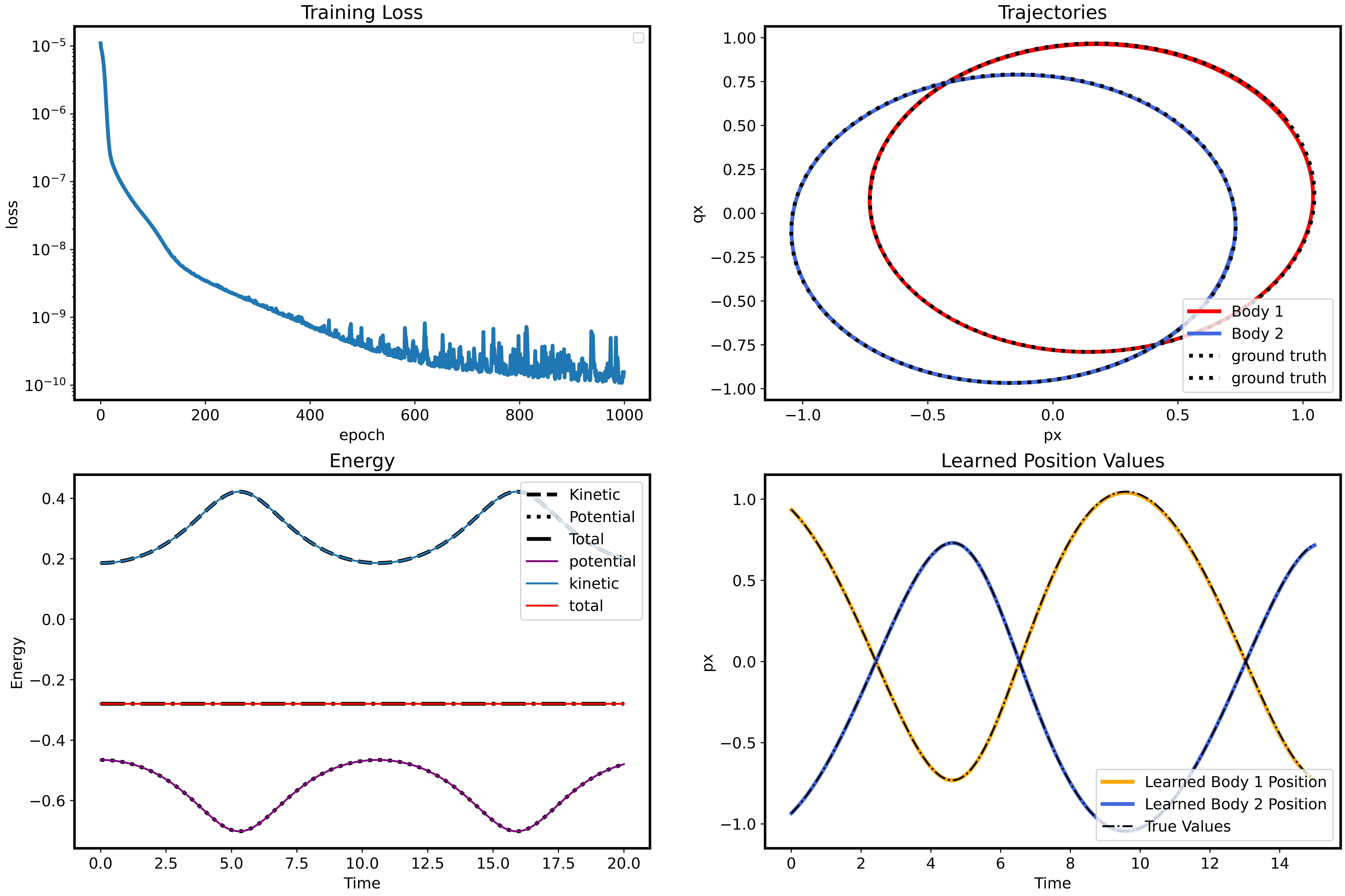
Figure 3 - Two Body Problem 1. Training Loss Graph 2. Learned Trajectories Graph over True Trajectories 3. Learned Energy over True Energy 4. Learned Position over True Position.
What’s Next
Currently our results look promising as our learned values closely match the ground truth values. Moving foward, we would like to add more complexity to our current examples: instead of fixed time steps, we would like to attempt variable time steps. We would also like to take on the Three Body Problem, which unlike our current examples has no analytical solution.
Information about Us
Mathias Heider is a rising senior at the University of Delaware, majoring in Computer Science and Mathematics and Economics. His interest are in machine learning and data science specifically when it relates to dataset with bioinformatics applications. Outside of class, Mathias likes to ski, hangout with friends, and play video games
Carrie Vanty is a rising senior at Middlebury College, majoring in mathematics. She loves working with ordinary differential equations in applied math. Outside of school, Carrie likes to ski, hike, and craft.
Emma Hayes is a rising junior at Carnegie Mellon University, majoring in Computational and Applied Mathematics. She enjoys learning about new topics in mathematics and incorporating computer science into her work. Outside of class, Emma likes hiking, baking, and making art.